
Excel SumProduct lookup multiple criteria not in first column
In this tutorial, I will explain how to use Excel SumProduct Function to lookup multiple criteria while the lookup value is not in first column of lookup range. The reason for writing this article is that Vlookup can only lookup one criteria and lookup value must be in the first column of lookup table.
You can also use Lookup Function to achieve the same result. Read the below article for details.
Excel Lookup Function lookup multiple criteria not in first column
You will also notice that SumProduct is very similar to SUMIFS and COUNTIFS, but
Syntax of SumProduct
SUMPRODUCT is to sum up the product of two or more arrays.
The syntax of SUMPRODUCT is
1- SUMPRODUCT(array1, array2, ...)
2- SUMPRODUCT(array1*array2* ...) OR
In formula 1, using a comma to separate different array follows the official syntax of SUMPRODUCT, however, it expects Number in each array. If they are not number, the product of Text returns 0. For example, TRUE*TRUE returns 0.
In formula 2, it does not follow the official syntax, but it is more flexible in multiplying Text. For the case TRUE*TRUE, the formula evaluates TRUE as 1 while FALSE as 0, and therefore TRUE*TRUE returns 1.
Based on the above characteristics, people put criteria in each array to test TRUE FALSE. The formula below is similar to using COUNTIFS.
1 - SUMPRODUCT(--array1=criteria1, --array2=criteria2, ...)  OR
2 - SUMPRODUCT((array1=criteria1)*(array2=criteria2) ...)
The double minus sign (–) is called double unary, it is to convert TRUE FALSE to 1 0, because array is expected to be number.
If you further product the result to a numerical array (arrray3), it becomes similar to using SUMIFS
1 - SUMPRODUCT(--array1=criteria1, --array2=criteria2, array3)  OR
2 - SUMPRODUCT((array1=criteria1)*(array2=criteria2)*array3)
For example, the below formula always return 0
=SUMPRODUCT({TRUE,TRUE,FALSE},{TRUE,TRUE,FALSE})
We can convert TRUE FALSE to 1 0 using double unary as below
=SUMPRODUCT(--{TRUE;TRUE;FALSE},--{TRUE;TRUE;FALSE})
=SUMPRODUCT({1;1;0},{1;1;0})
= 1*1 + 1*1 + 0*0
= 2
Alternatively, simply use asterisk as formula 2
=SUMPRODUCT({TRUE;TRUE;FALSE}*{TRUE;TRUE;FALSE})
=SUMPRODUCT({1;1;0},{1;1;0})
= 1*1 + 1*1 + 0*0
= 2
Difference between SUMIFS and SUMPRODUCT, COUNTIFS and SUMPRODUCT
Syntax of SUMIFS
SUMIFS(sum_range, criteria_range1, criteria1, [criteria_range2, criteria2], ...)
Syntax of COUNTIFS
COUNTIFS(criteria_range1, criteria1, [criteria_range2, criteria2]…)
Apart from the syntax difference, one major difference is that criteria in the above two formula require Text, which means you have to double quote the criteria. This makes the criteria difficult because you cannot easily input a formula in a criteria because it will be considered as a Text. Instead, you have to use & sign to split the real Text and formula.
The below example shows how you present your criteria by joining Text and Reference.
=COUNTIFS(A1:A5,">=3",B1:B5,">=" &A7&+MONTH(TODAY()))
In SumProduct, you just need to directly apply formula and reference, much more simple
=SUMPRODUCT((A1:A5>=3)*(B1:B5>=A7+MONTH(TODAY())))
The second difference is that you cannot transform the array data, but you can do it in SUMPRODUCT.
In COUNTIFS, the following formula will fail
=COUNTIFS(Month(A1:A5),">=3"...
But in SUMPRODUCT, the following formula will work
=SUMPRODUCT(Month(A1:A5)>=3...
In conclusion, for single criteria, you should use COUNTIF and SUMIF, but for multiple criteria, you should definitely use SUMPRODUCT (because SUMPRODUCT cannot use on single criteria).
SUMPRODUCT with OR condition
In normal formula, you can use OR keyword to test TRUE or FALSE or two criteria. For example
=If(OR(A1=”Resignation”,A1=”Termination”),1,0)
In SUMPRODUCT, the you can sum up the two array directly, because if one of them is true it becomes 1+0 or 0+1, the result becomes 1.
=SUMPRODUCT(((A1:A5=”Resignation”)+(A1:A5=”Termination”))*B2:B5)
Assumption of Example – lookup multiple criteria
In the above sections, I have explained the logic of SUMPRODUCT, now we come to a real example.
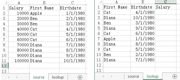
In this example, we have two worksheets:
1) source – the source table being looked up
2) lookup – the lookup table in which you want to lookup salary from source
First Name and Bbirthdate are keys to identify an unique person.
Example of SUMPRODUCT – lookup multiple criteria
In worksheet “lookup”, fill in column C with formula as show in column D.

Lets take a look at the formula in D2, I highlight the three different arrays using different colors below.
=SUMPRODUCT((source!$B$2:$B$11=lookup!A2)*(source!$C$2:$C$11=lookup!B2)*source!$A$2:$A$11)
For the first array in red, we try to test if First Name = Cat, if TRUE return 1, otherwise return 0.
For the second array in green we try to test if Birthdate = 29224 (4/1/1980), if TRUE return 1, otherwise return 0.
For the third array in purple, we product salary in source table, not checking anything.
The mechanism of the formula in D2 is explained below. Note that Birthdate is converted to time serial value in calculation.
=SUMPRODUCT((source!$B$2:$B$11=lookup!A2)*(source!$C$2:$C$11=lookup!B2)*source!$A$2:$A$11)
=SUMPRODUCT({"Apple";"Ben";"Ben"; ... ="Cat"}*{29221;29222;29223;...=29224}*{10000,20000,30000;...})
=SUMPRODUCT({0;0;0;1;1;1;0;0;0;0}*{0;0;0;1;0;0;0;0;0;0}*{10000,20000,30000;40000;50000;60000;70000;80000;90000;100000})
=SUMPRODUCT({0;0;0;1;0;0;0;0;0;0}*{10000,20000,30000;40000;50000;60000;70000;80000;90000;100000})
= 0*10000+0*20000+0*30000+1*40000+0*50000+0*60000+0*70000+0*80000+0*90000+0*100000
=40000
Two points to note:
1) You must assume the key combination (First Name and Birthdate) is unique in worksheet “source”, otherwise all salary of that key will sum up in the result.
2) This method only works assume that the lookup result (Salary) is numeric, because SUMPRODUCT can only product value but not text. For example, the below formula return #VALUE!
=SUMPRODUCT({0;0;0}*{"A",20000,30000})
Use SUMPRODUCT, INDEX and ROW to return text result
Syntax of INDEX Function
INDEX( array, row_number, [column_number] )
| array | A range of cells or table. |
| row_number | The row number in the array to use to return the value. |
| column_number | zoptional. It is the column number in the array to use to return the value. |
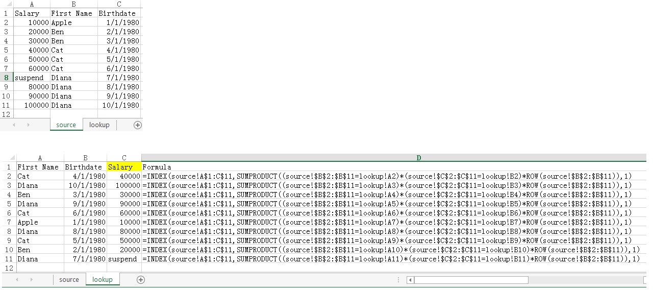
In order to return text result using SumProduct, first we multiply the condition arrays by row number, and then use the returned value as column parameter of INDEX Function.
The mechanism of the formula in C2 is explained below. Note that Birthdate is converted to time serial value in calculation.
=INDEX(source!A$1:C$11,SUMPRODUCT((source!$B$2:$B$11=lookup!A2)*(source!$C$2:$C$11=lookup!B2)*ROW(source!$B$2:$B$11)),1)
=INDEX(source!A$1:C$11,SUMPRODUCT({"Apple";"Ben";"Ben"; ... ="Cat"}*{29221;29222;29223;...=29224}*{2;3;4;...}),1)
=INDEX(source!A$1:C$11,SUMPRODUCT({0;0;0;1;1;1;0;0;0;0}*{0;0;0;1;0;0;0;0;0;0}*{2;3;4;5;6;7;8;9;10;11}),1)
=INDEX(source!A$1:C$11,SUMPRODUCT({0;0;0;1;0;0;0;0;0;0}*{2;3;4;5;6;7;8;9;10;11}),1)
=INDEX(source!A$1:C$11,0*2+0*3+0*4+1*5+0*6+0*7+0*8+0*9+0*10+0*11,1)
=40000
Outbound References
http://blogs.office.com/2012/04/26/using-multiple-criteria-in-excel-lookup-formulas/