This SPSS Excel tutorial explains how to run Multiple Regression in SPSS and Excel.
You may also want to read:
Multiple Regression (Multiple Linear Regression)
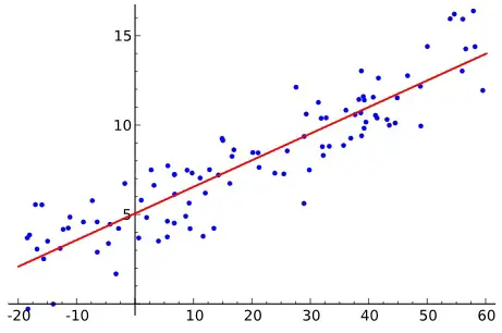
Regression analysis is to predict the value of one interval variable based on another interval variable(s) by a linear equation. We draw a random sample from the population and draw the best fitting straight line in order to estimate the population. The straight line is known as least squares or regression line.
If the linear regression model only has one independent variable, we call it simple linear regression. For multiple independent variables, we call it multiple regression (multiple linear regression).
The regression line equation of multiple linear regression is represented as
y = bo + b1x1 + b2x2 + ... bkxk
where
y is the dependent variable
bo is the intercept
bn is the coefficient of independent variable
xk is the independent variable
Multiple Regression – Excel
Before we begin, make sure you have installed Analysis Toolpak Add-in
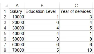
Assume we want to study how education level and year of services relate to salary.
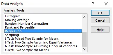
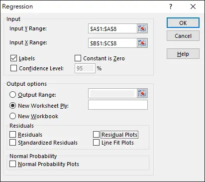
Navigate to DATA tab > Data Analysis > Regression > OK
Select the data Range as below. Note that X Range is the independent variable while Y Range is the dependent variable.
Click on OK.
The result is generated.
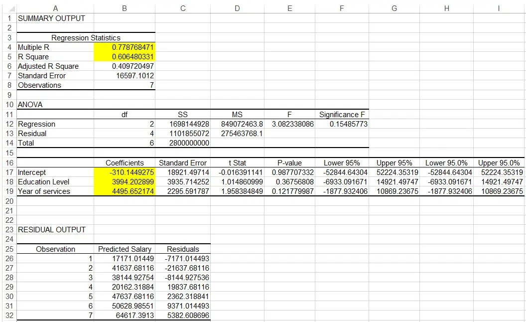
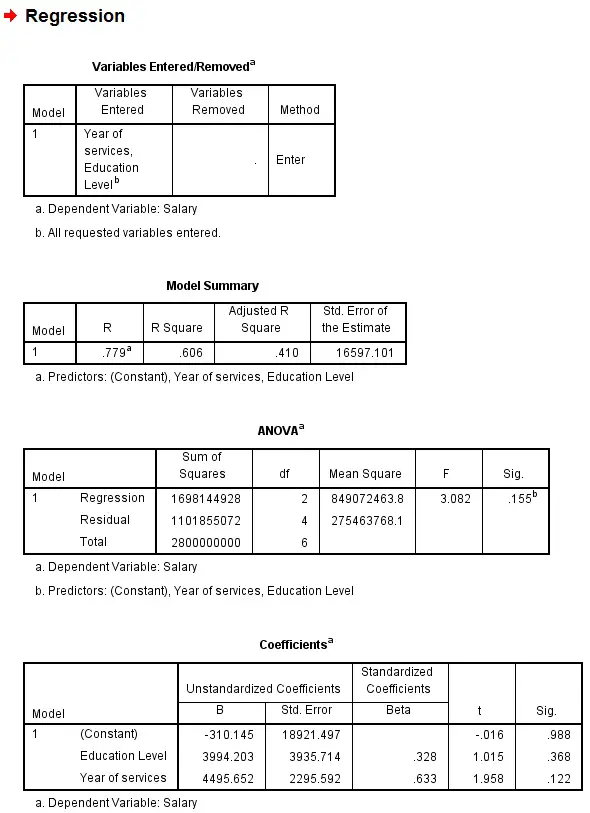
Regression Statistics Table
Multiple R is known as Multiple Coefficient of Correlation, which measures the strength of the correlation. +1 is a linear relation, 0 is no relation, -1 is negative linear relation. In our example, 0.78 shows a strong positive relation.
R Square is known as Coefficient of Determination, it measures how many percentage of variation in Y can be explained by variation in X. In our example, 61% of variation in salary can be explained by variation in education level and year of services.
ANOVA Table
This table is to test the significance of the Regression model, which is >0.05 in our example (not significant)
The 3rd table
Coefficients of Intercept means the Intercept, while coefficient of education is b1, coefficient of year of services is b2, therefore the regression line is
Y = -310 + 3994x1 + 4995x2
Residual Output Table
This table shows the difference between the observation and the predicated values, Residuals is the difference.
We take the 10000 salary observation as an example.
We substitute x1 = 1, x2 = 3 into the regression model
Predicted value = -310 + 3994x1 + 4995x2
= -310 + 3994(1)+ 4995(3)
= 17171
Residual = observation value – predicted value
= 10000 – 17171
= -7171
Another important value is P-value, it shows that how significant of each factor is in the Regression model. In our example, P value of year of services is 0.12, which is larger than 0.05, meaning Year of Services is not a strong predictor in salary.
Multiple Regression – SPSS
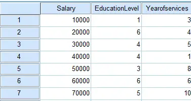
Prepare data source as below
Navigate to Analyze > Regression > Linear (Multiple Regression is actually a Multiple Linear Regression)
Select Dependent variable and Independent variable as below > OK
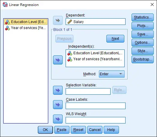
The result is generated as below. The results and the structures are basically the same as the Excel output.