This tutorial explains how to use Excel Rank Function to give a number a rank in a range of number.
Syntax of Rank Function
RANK(number,ref,[order])
| Number | Required. The number whose rank you want to find. |
| Ref | Required. An array of, or a reference to, a list of numbers. Nonnumeric values in ref are ignored. |
| Order | Optional. A number specifying how to rank number. If order is 0 (zero) or omitted, Microsoft Excel ranks number as if ref were a list sorted in descending order. If order is any nonzero value, Microsoft Excel ranks number as if ref were a list sorted in ascending order. |
Example of Rank Function
Assume that we have a list of numbers from A1 to A10
| Formula | Result | Explanation |
| =RANK(A4,A1:A10) | 7 | The rank of number 4 in descending order of number 1 to 10 |
| =RANK(A4,A1:A10,1) | 4 | The rank of number 4 in ascending order of number 1 to 10 |
Note that if the two numbers to be ranked are the same, then the rank of the two numbers are the same, and the next rank will be skipped.
For example, if values of A1 and A2 are 1, then in the ascending ranking, both A1 and A2 rank 1, but A3 will rank 3 instead of rank 2.
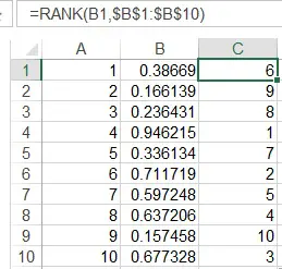
Assign random number to values
You may use Rand() Function in column B and then assign unique number in column C using Rank Function.
For details, please click
Assign unique random number using Excel
Outbound References
https://support.office.com/en-us/article/RANK-function-6a2fc49d-1831-4a03-9d8c-c279cf99f723


