Excel VBA freeze panes using FreezePanes property

This Excel tutorial explains how to freeze panes in Excel spreadsheet and freeze panes in Excel VBA using FreezePanes property.

Freeze Panes in Excel spreadsheet

To explain how to freeze panes in Excel VBA, first I have to explain how to freeze panes in Excel spreadsheet.

Freeze Row

The most common kind of freeze panes is to freeze the first row as it contains the header of the column. So that when you scroll down the spreadsheet, you can still see the header in row 1.

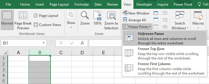
Highlight row 2, navigate to View > Freeze Panes > Freeze Panes

Similarly, you can freeze row 2 by highlighting row 3 (highlight one row down the frozen row).

Freeze Column

To display data all the time in column A when you scroll to the right of the spreadsheet, highlight column B, , navigate to View > Freeze Panes > Freeze Panes

Similarly, you can freeze column A and B by highlighting column C (highlight the right column of the target frozen column).

Freeze Row + Column

To freeze column A and row 1 at the same time, select column B2, navigate to View > Freeze Panes > Freeze Panes

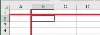
In the screenshot, I have highlighted the direction of freeze of a selected cell, it is the top row and left column of a selected Cell.

Freeze Panes in Excel VBA

Similar to freeze panes in Excel spreadsheet, to freeze panes in Excel VBA, select a Cell first, then set ActiveWindow.FreezePanes Property to TRUE.

Freeze Row

To freeze row 1, select Row 2. Setting FreezePanes to False is to ensure that we have unfrozen any active freezePanes first. FreezePanes won’t work if there is already a FreezePanes.

Sub FreezeRow()
   ActiveWindow.FreezePanes = False
   Rows("2:2").Select
   ActiveWindow.FreezePanes = True
End Sub

Freeze Column

To freeze column A, select column B.

Sub FreezeColumn()
   ActiveWindow.FreezePanes = False
   Columns("B:B").Select
   ActiveWindow.FreezePanes = True
End Sub

Freeze row + column

To freeze column A and row 1, select Cell B2.

Sub FreezeCell()
   ActiveWindow.FreezePanes = False
   Range("B2").Select
   ActiveWindow.FreezePanes = True
End Sub

Unfreeze Panes

To unfreeze panes, simply set the FreezePanes Property to False.

   ActiveWindow.FreezePanes = False

Use Split to freeze Panes in Excel VBA

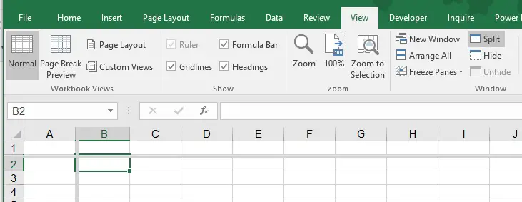
Instead of selecting a Cell to determine the freeze panes, we can also apply Split first, and then Set FreezePanes to TRUE.

For example, in order to freeze column A and row 1, write VBA code to split column 1 Row 1, afterwards set the ActiveWindow.FreezePanes to TRUE.

Sub FreezeCell()
    With ActiveWindow
    .SplitColumn = 1
    .SplitRow = 1
    End With
    ActiveWindow.FreezePanes = True
End Sub