This Excel tutorial explains how to Vlookup different format (a mix of text and number).
You may also want to read:
Excel verify Text format and convert number to text
Excel verify number format and convert Text to Number
Issue with VLookup different format (a mix of text and number)
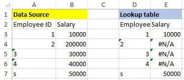
Sometimes your data source table may contain a mix of text and number, let’s say Employee ID in column A.
In the Lookup table, when your lookup value (column D) are all number, you will fail to lookup the text values in column A.
Similarly, when your lookup value in column D are all text, you will fail to lookup the number in column A.
The last case is that the Employee ID in column D are already a mix of number and text.
Solution of VLookup different format (a mix of text and number)
In order to vlookup different format, the first step is to try to lookup the original value as you normally do.
In Cell E3, type the below formula
=VLOOKUP(D3,$A$3:$B$7,2,0)
We have the below result with 3 #N/A
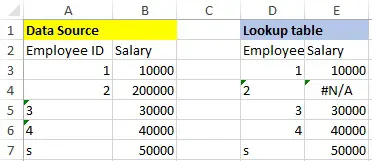
To fix the #N/A, use IFERROR Function to capture the #N/A cases. We try to convert column A number to text to see if we can vlookup more cases. To do the conversion trick, use &”” after the cell
Update the below formula in D2.
=IFERROR(VLOOKUP(D3,$A$3:$B$7,2,0),VLOOKUP(D3&"",$A$3:$B$7,2,0))
Now we get the result with only one #N/A left.
To deal with the last #N/A due to type mismatch, we convert D4 from text to number by multiplying D2 with a dummy value 1.
Now update D2 again with one additional IFERROR.
=IFERROR(IFERROR(VLOOKUP(D3,$A$3:$B$7,2,0),VLOOKUP(D3&"",$A$3:$B$7,2,0)),VLOOKUP(D3*1,$A$3:$B$7,2,0))
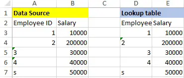
We successfully all values with no #N/A.
An alternative would be using Value Function to convert text to number as below.
=IFERROR(IFERROR(VLOOKUP(D3,$A$3:$B$7,2,0),VLOOKUP(D3&"",$A$3:$B$7,2,0)),VLOOKUP(VALUE(D3),$A$3:$B$7,2,0)


