Change Pivot Table Layout, why?
To illustrate why we want to change Pivot Table Layout, lets see the below example.
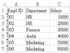
Assume that we use the following data to create a Pivot Table. We want to show the total summary, group by Department, Empl ID.
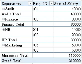
Excel 2003 – Tabular layout
Pivot Table layout is called “Tabular”, where each grouping is in one column, and the subtotal is at the bottom of each group.
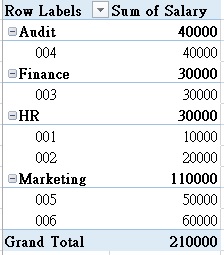
Excel 2007 and onwards – Compact layout
By default, Pivot Table layout is called “Compact”, where groupings are in one column, and subtotal is on top of each group.
Even worse, the column label “Department” and “Empl ID” are gone.
I personally hate this layout because it does not use the actual column name, instead it uses “Row Labels”, “Column Labels”.
Since “Row Labels” refer to both Department and Empl ID as they display in one column, it uses a generic name “Row Labels”.
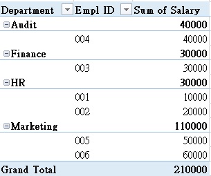
Excel 2007 and onwards – Outline layout
There is another new layout called “Outline”, where the layout format is between “Tabular” and “Compact”.
Change Pivot Table Layout using VBA
Before continue reading, you should have knowledge in creating Pivot Table using VBA. If not, read the below article first
Create Pivot Table using Excel VBA
You can change the layout using VBA Code
ActiveSheet.PivotTables("PivotTable1").RowAxisLayout xlOutlineRow
ActiveSheet.PivotTables("PivotTable1").RowAxisLayout xlTabularRow
ActiveSheet.PivotTables("PivotTable1").RowAxisLayout xlCompactRow
Alternatively, you can define Version and DefaultVersion when you create Pivot Cache and Pivot Table using VBA. Note that version for Pivot Cache and Pivot Table has to be the same, otherwise you will receive the following error.
Run-time error ‘5’: Invalid procedure call or argument
Syntax of PivotCaches and CreatePivotTable
PivotCaches.Create(SourceType, SourceData, Version)
CreatePivotTable(TableDestination, TableName, ReadData, DefaultVersion)
The DefaultVersion of Excel 2013 is xlPivotTableVersion15 while Excel 2003 is xlPivotTableVersion10. (Version10 is what I tested in Excel 2003 although the below table from MSDN shows Version11, but they should have no difference)
| Name | Value | Description |
| xlPivotTableVersion2000 | 0 | Excel 2000 |
| xlPivotTableVersion10 | 1 | Excel 2002 |
| xlPivotTableVersion11 | 2 | Excel 2003 |
| xlPivotTableVersion12 | 3 | Excel 2007 |
| xlPivotTableVersion14 | 4 | Excel 2010 |
| xlPivotTableVersion15 | 5 | Excel 2013 |
| xlPivotTableVersionCurrent | -1 | Provided only for backward compatibility |
Below is an example to create a 2003 version Pivot Table in Excel 2013
    ActiveWorkbook.PivotCaches. _
        Create( _
        SourceType:=xlDatabase, _
        SourceData:=Worksheets("Sheet1").Range("A1:B7"), Version:=xlPivotTableVersion10). _
            CreatePivotTable _
            TableDestination:=Worksheets("Sheet5").Range("A1"), _
            TableName:="PivotTable1", DefaultVersion:=xlPivotTableVersion10
Rename RowLabels and ColumnLabels of Compact Layout
You can change any label in the Pivot Table.
To change RowLabels and Column Labels
ActiveSheet.PivotTables("PivotTable1").CompactLayoutRowHeader = "NewRowName"
ActiveSheet.PivotTables("PivotTable1").CompactLayoutColumnHeader = "NewColumnName"
To change “Grand Total”
ActiveSheet.PivotTables("PivotTable1").GrandTotalName = "NewGrandTotal"
To change name of Pivot Items
Any other names you see in the Pivot Table are called “Pivot Items” (such as Department name, Empl ID), the name can be changed through Caption Property.
Below example shows how to change the Pivot Items “Sum of Salary” to “NewSumOfSalary”.
ActiveSheet.PivotTables("PivotTable1").DataPivotField.PivotItems("Sum of Salary").Caption = "NewSumOfSalary"
What’s next?
Now you have created a Pivot Table, and changed the layout you want. The next step is to play around with Filters in VBA. You are recommended to read the article.
Excel VBA multiple criteria for Label Filter of Pivot Table
Outbound References
http://msdn.microsoft.com/en-us/library/office/ff837609%28v=office.15%29.aspx


