This Excel tutorial explains how to check duplicate values in Excel spreadsheet by highlighting duplicate values using Conditional Formatting.
You may also want to read:
Excel assign sequence number to duplicate records
Excel delete duplicated data in consecutive rows
Excel check duplicate values
Back in Excel 2003, it was a pain to identify duplicate values. What I used to do was to sort the values in ascending order and then added an assist column to check if the value on the left equals to the next cell value, then filter “TRUE”. Since Excel 2007, Excel introduced a new Conditional Formatting option to highlight duplicate values in specific color, and then you can apply a Filter in the value column to filter the highlighted cells.
Let’s say we have generated a staff list, and we want to verify if the staff list contains duplicate employee ID to ensure only one employee ID for one staff. Duplicate usually happens when you try to join two tables but they have One to Many Relationship or Many to Many Relationship.
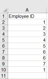
Highlight the column you want to check duplicate values.
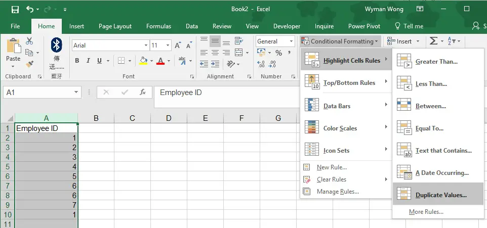
Navigate to Home tab > Conditional Formatting > Highlight Cells Rules > Duplicate Values
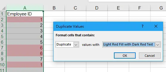
Select color for duplicate values in the dropdown box. Now that you can see all duplicate values are highlighted in pink.
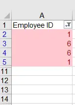
In order to quickly filter all duplicate values, add a Filter to the column (Data tab > Filter) , then select Filter by Color > select the color
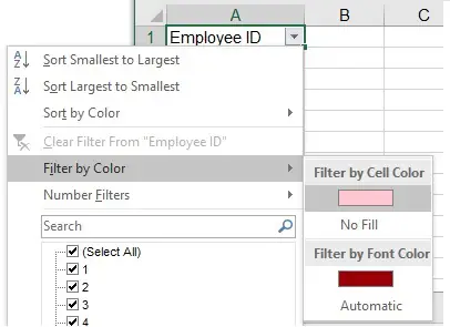
Only duplicate values are displayed