This Excel tutorial explains how to use Excel IFERROR function for worksheet. IFERROR can be used with vlookup to capture ISNA error.
You may also want to read:
Check Excel #N/A using ISNA Function
What is Excel IFERROR Function?
Excel IFERROR Function is an error handling function, if an “Error” is found, then a desired value is returned. This is a new function introduced in Excel 2007, which means Excel 2003 and prior versions cannot be used.
Syntax of IFERROR
IFERROR(value,value_if_error)
The types of errors that can be captured are shown in the below table.
| #N/A |
| #VALUE! |
| #REF! |
| #DIV/0! |
| #NUM! |
| #NAME? |
| #NULL! |
Example of Excel IFERROR
One common use of IFERROR function is to use with Vlookup. If a lookup value is not found, Vlookup function returns #N/A
In Excel 2003, we used to use ISNA or ISERROR to capture the error.
=IF(ISNA(VLOOKUP(xxxx)),"Not found",VLOOKUP(xxxx))
OR
=IF(ISERROR(VLOOKUP(xxxx)),"Not found",VLOOKUP(xxxx))
In Excel 2007 and newer version, because IFERROR has combined functions “IF” and “ISERROR”, we can simplify the formula as
=IFERROR(VLOOKUP(xxxx),”Not found”)
Although many people use IFERROR nowadays, you should be very careful that you will also turn other errors, not just those values you fail to lookup.
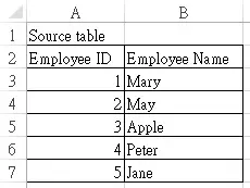
For example, we tried to look up Employee ID from the below source table.
| Employee ID | Formula | Result |
| 1 | =IFERROR(VLOOKUP(D3,$A$3:$B$7,2,0),”Not found”) | Mary |
| 6 | =IFERROR(VLOOKUP(D4,$A$3:$B$7,2,0),”Not found”) | Not found |
| 7 | =IF(ISNA(VLOOKUP(D5,$A$3:$B$7,2,0)),”Not found”,VLOOKUP(D5,$A$3:$B$7,2,0)) | Not found |
| 8 | =IF(ISERROR(VLOOKUP(D5,$A$3:$B$7,2,0)),”Not found”,VLOOKUP(D5,$A$3:$B$7,2,0)) | Not found |
Outbound References
http://www.excelfunctions.net/Excel-Iferror.html

