
This Excel tutorial explains how to select specific columns in a worksheet with many columns using Custom Views and Query.
You may also want to read:
Create Excel Query and update Query
Excel automatically select specific columns using Custom Views and Query
Many people including myself like creating a master report with many columns and then send it to users for them to manually select columns they need. The reason is that it is time consuming to customize a lot of reports and it is difficult to maintian when report conditions update. With a single source of data, we can simply maintain the master report.
However, many users complain that there are too many columns in the report that they do not need. To cope with this difficulty, Excel Custom Views function allows useres to select specific columns to save as a template. So everytime they receive the master files, the columns can be automatically selected.
You can also use Custom Views to save hidden rows, filter, window settings, print settings, print areas. The focus of this post is to demonsate how to hide columns.
Create Custom Views
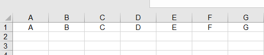
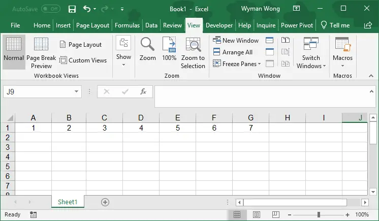
Lets say we have a master file with columns A to G. Now we want to select column A C F only.
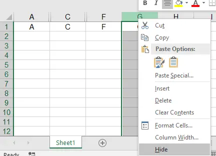
Manually Hide columns B D E G
Select View Tab > Custom Views > Add
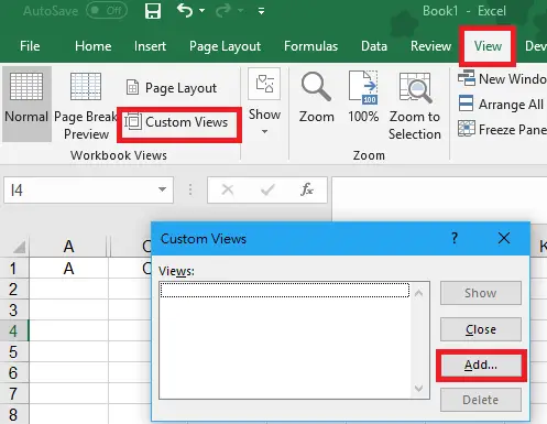
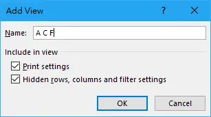
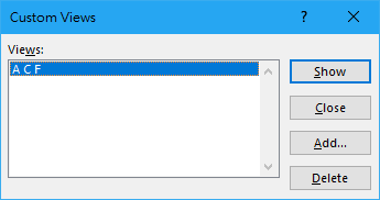
Type a name for the View > OK
Apply Custom Views
Let’s say you receive the master list in the next month. Copy the contents from the master list to the exact worksheet that you previously set Custom Views. Custom Views won’t work your data is not in the worksheet which you created Custom Views for. It also doesn’t work if you delete the original worksheet and then rename to the same worksheet name.
Navigate to View tab > Custom Views > Show
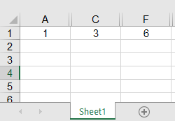
Only columns A C F are displayed.
Select specific columns using Query
Another better solution to automatically select specific columns is to create a Query in Excel. The reason is that Query recognizes the column header name to select, not the actual column order such as A B C. You may refer to the details in my previous post on how to create Excel Query, but I will quickily demonstrate how to do it in this post.
Let’s say we have saved the master list on the Desktop.
Create a new workbook, select Data tab > from Other Sources > from Microsoft Query

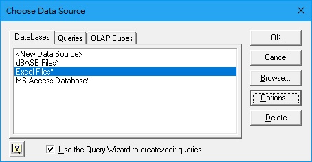
Select Excel Files > OK
Select the master list location to import, then select field headers 1, 3, 6
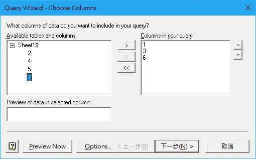
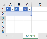
Select next step until finish. Now columns 1, 3, 6 are imported.
Now whenever you update the master list, refresh this Table (Data > Refresh All) to get the latest dta from master list.
If you are unable to refersh the data, go to Trust Center Settings to configure the Trusted Location and Extenal Content.
Outbound References
