
Excel Lookup Function lookup multiple criteria not in first column
In this tutorial, I will explain how to use Excel Lookup Function to lookup multiple criteria while the lookup value is not in first column of lookup range. The reason for writing this article is that Vlookup can only lookup one criteria and lookup value must be in the first column of lookup table.
You can also use SUMPRODUCT Function to achieve the same result in the below article.
Excel SumProduct lookup multiple criteria
Syntax of Lookup Function
LOOKUP(lookup_value, lookup_range, result_range)
| lookup_value | Required. A value that LOOKUP searches for in the first vector |
| lookup_range | Required. A range that contains only one row or one column |
| result_range | Optional. A range that contains only one row or column. |
If the LOOKUP function can not find an exact match, it chooses the largest value in the lookup_range that is less than or equal to the value. We will make use of this property in lookup multiple criteria.
Example of Lookup Function – lookup multiple criteria
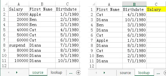
In this example, we have two worksheets:
1) source – the source table being looked up
2) lookup – the lookup table in which you want to lookup salary from source
First Name and Bbirthdate are keys to identify an unique person.
Now apply the lookup formula as below in column C. Column D is to show the actual formula of column C.
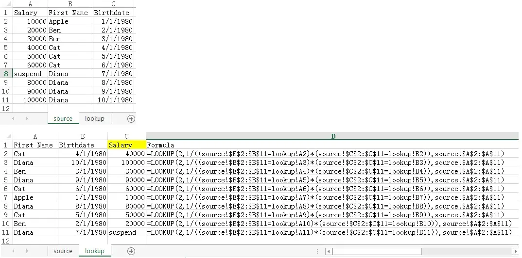
Explanation of Formula – lookup multiple criteria
Let’s take a look at the formula at D2
=LOOKUP(2,1/((source!$B$2:$B$11=lookup!A2)*(source!$C$2:$C$11=lookup!B2)),{10000;20000;30000;...})
| Parameter name | Parameter value |
| lookup_value | 2 |
| lookup_range | 1/((source!$B$2:$B$11=lookup!A2)*(source!$C$2:$C$11=lookup!B2)) |
| result_range | source!$A$2:$A$11 |
Below is the mechanism of the formula.
=LOOKUP(2,1/((source!$B$2:$B$11=lookup!A2)*(source!$C$2:$C$11=lookup!B2)),source!$A$2:$A$11)
=LOOKUP(2,1/({Apple;Ben;Ben;Cat;...="Cat"}*{29221;29222;29223;29224;...=29224}),{10000;20000;30000;40000;...})
=LOOKUP(2,1/({FALSE;FALSE;FALSE;TRUE;...}*{FALSE;FALSE;FALSE;TRUE;...}),{10000;20000;30000;40000;...})
=LOOKUP(2,1/{0;0;0;1;...},{10000;20000;30000;40000;...})
=LOOKUP(2,{#DIV/0;#DIV/0;#DIV/0;1;...},{10000;20000;30000;40000;...})
=40000
In the second parameter
1/{0;0;0;1;…}
The reason for dividing an array by 1 is that we want to turn all “0” to non numerical value (i.e. error)
{#DIV/0;#DIV/0;#DIV/0;1;...}
Afterwards, we apply LOOKUP formula and use “2” as the lookup_value parameter, where “2” is a constant that can be applied to other formula. When we lookup a value (2) which cannot be found in the array (a combination of 1 and #DIV/0), the Function will match the largest value (1) in the lookup_range (1 and #DIV/0) that is less than or equal to the value (2). In fact, you can also use “1” as the lookup_value parameter assume that value 1 can be found in the array, the Function will return the last matched value as well. As a normal practice, people tend to use “2” as parameter.
Outbound References
http://blogs.office.com/2012/04/26/using-multiple-criteria-in-excel-lookup-formulas/