
This Excel tutorial explains how to interpret the summary table generated from Excel Descriptive Statistics.
Excel Descriptive Statistics
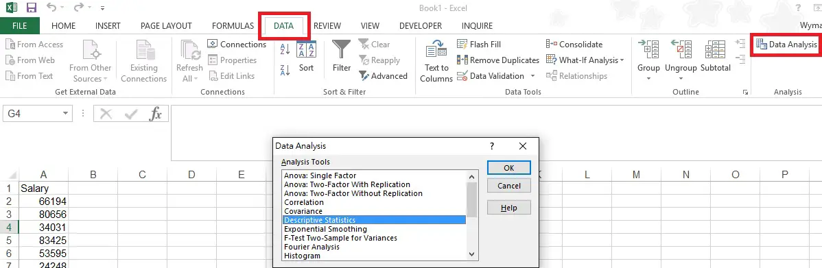
One of the options under DATA > Data Analysis is Descriptive Statistics, which generates a statistics summary of a variable. It is very useful because it saves you a lot of time from entering a lot of formulas in order to get some basic analysis.
Before using Excel Descriptive Statistics feature, you should first install Analysis Toolpak Add-Ins.
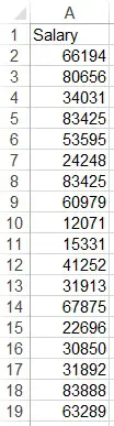
Assume that you want to analyze the salary of the employees. (I used RandBetween Function to generate the random numbers)
Navigate to DATA > Data Analysis > Descriptive Statistics
Select Input Range as A1:A19 and check the box Labels in first row, so that the summary table header will display the name “Salary”.
Follow other options as below, click on OK.

A new worksheet is created for the below summary table.
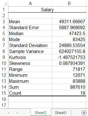
Below are the meaning of each item.
| Item | Description | Equivalent Formula |
| Mean | Average of the values | =AVERAGE(Sheet1!A2:A19) |
| Standard Error | Standard deviation of the sample mean | =STDEV.S(Sheet1!A2:A19) / SQRT(COUNT(Sheet1!A2:A19)) |
| Median | Rank data from lowest to highest (or highest to lowest), the number in the middle | =MEDIAN(Sheet1!A2:A19) |
| Mode | The most frequent occurrence | =MODE(Sheet1!A2:A19) |
| Standard Deviation | Sample standard deviation, measure how close the data is to the mean. 0 means very close to the mean | =STDEV.S(Sheet1!A2:A19) |
| Sample Variance | Square of standard deviation | =VAR.S(Sheet1!A2:A19) |
| Kurtosis | Measure the flatness of the distribution. Positive kurtosis indicates a relatively peaked distribution.Negative kurtos is indicates a relatively flat distribution. |
=KURT(Sheet1!A2:A19) |
| Skewness | Skewness is a measure of symmetry. Sk = 0 means frequency distribution is normally distributed. Positive Sk means positively skewed, negative Sk means negatively skewed. | =SKEW(Sheet1!A2:A19) |
| Range | Largest value minus smallest value | =MAX(Sheet1!A2:A19)-MIN(Sheet1!A2:A19) |
| Minimum | Smallest value | =MIN(Sheet1!A2:A19) |
| Maximum | Largest value | =MAX(Sheet1!A2:A19) |
| Sum | Sum of all values | =SUM(Sheet1!A2:A19) |
| Count | Count of all values | =COUNT(Sheet1!A2:A19) |
At the bottom of the Descriptive Statistics box, there are three additional options.
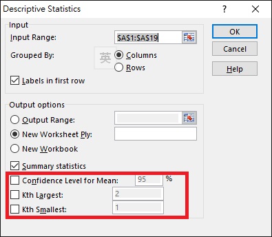
Confidence Level for the Mean
Confidence level is the percentage that the value will fall into the range. Using our example, if we input 95% as confidence level, the generated value is 12422, meaning 95% chance that the values fall from sample mean – 12422 to sample mean + 12422 (from 36889 to 61734).
You can use CONFIDENCE Function to get the same result. Note that 95% is converted to 0.05 (1-0.95) in the first argument.
=CONFIDENCE.T(0.05,STDEV.S(Sheet1!A2:A19),18)
Kth Largest / Kth Smallest
The meaning is self explanatory. For example, if we input 2 for Kth Largest, which means we want to find the second largest value, and the summary table will show an additional row
| Largest(2) | 83425 |
Kth Smallest on the other hand, finds the Kth smallest number.