This Excel tutorial explains how to find last row using Excel worksheet formula.
Excel find the last row
Finding the last row in Excel is very important especially for creating dynamic data Range, which can be used for setting dynamic Print Area, dynamic Data Validation list, dynamic data source for Pivot Table, etc.
When you google this topic, most article talks about how to find the last row using VBA but not the non-VBA solution. In my previous post I have also detailed different ways to find the last row and last column using Excel VBA. This tutorial explains how to find the last row using worksheet formula without using VBA.
Find the last row using Worksheet Formula
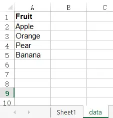
Assume that you have the below fruit list.

Find Last Row Number
The below formula looks for the last row number in column A.
=SUMPRODUCT(MAX((data!$A:$A<>"")*ROW(data!$A:$A)))
This formula returns 5
There are several solutions in the internet using COUNTA Function, COUNT Function and other formulas but they have different limitations. This one uses MAX Function and ROW Function, which is probably the best choice.
If you are just trying to use this formula without understanding the logic, you can simply replace the column number “A” with the column you want to check.
If you want to understand more, please read my previous post on the use of SUMPRODUCT Function to multiply two Array.
Find Last Row Value
The below formula looks for the last row value in column A. This formula is based on the previous one and uses INDIRECT Function to convert row number back to a Range.
=INDIRECT("A"&SUMPRODUCT(MAX((data!$A:$A<>"")*ROW(data!$A:$A))))
This formula returns Banana
Find Data Range up to last row data
The below formula select Range A1 to the last row in column A. The key of this formula is to set a data Range using OFFSET Function.
=OFFSET(data!$A$1,0,0,SUMPRODUCT(MAX((data!$A:$A<>"")*ROW(data!$A:$A))),1)
You can use this trick to create Name Range for setting dynamic Print Area, dynamic Data Validation list.
