Excel Lookup Function lookup multiple criteria

This Excel tutorial explains how to use Excel Lookup Function and how to look up multiple criteria.

You may also want to read:

Excel Vlookup second matched value or specific occurence

Excel Lookup Function lookup multiple criteria not in the first column

Excel lookup partial text using Vlookup with Wildcard

Excel Lookup Function – lookup multiple criteria

Excel Lookup Function is to look up a value in a Range (or array) and return the corresponding result in another Range (or array). Note that “Range” is also known as “Vector” if you read other tutorial.

Differences between Lookup and Vlookup

First of all, lets recap the syntax of Vlookup

VLOOKUP(lookup_value, table_array, col_index_num, [range_lookup])

Lookup Function behaves similarly as Vlookup if the last parameter [range_lookup] of vlookup is set to TRUE.

TRUE means to look for similar match, FALSE means to look for exact match. It is not helpful to look for similar match in 99% situations because it may not return the exact result we want. In Lookup Function, we cannot choose to look for exact match or similar match, we can only look for similar match.

In order to make an apple to apple comparison, I will talk about how Lookup behaves differently against Vlookup with FALSE [range_lookup] below.

1 – For Lookup Function, lookup Range must be in ascending order. Vlookup (last Function parameter =FALSE) does not have such requirement.

2 – Lookup Function can look up value not in the first column of lookup Range, because you can specify the lookup Range anywhere instead of specifying the Nth column in lookup table

3 – If there are more than one matched results, Vlookup (last Function parameter =FALSE) returns the first matched value, while Lookup returns the last matched value

3 – If Lookup Function cannot find an exact match, it returns the largest value in the lookup Range that is less than or equal to the lookup value (behave the same way as Vlookup when the last parameter is set to TRUE). While you can easily identify which is larger for numeric value (for example, 1000 > 10).

For text like alphabets or symbols, the comparison is based on ASCII value of the text (for example, a> A >?> 1), read the references at the bottom of the post for ASCII value and text conversion.

Therefore even if there is no match, Lookup Function may still return a value, while Vlookup returns #N/A.

Syntax of Lookup Function

LOOKUP(lookup_value, lookup_range, result_range)

lookup_value	A Range or array that LOOKUP searches for
lookup_range	A lookup Range or array that contain only one row or one column, must be sorted in ascending order
result_range	Optional. A range that contains only one row or column.

Click here to see the detailed explanation.

Example of Lookup Function

In this example, we have two worksheets:

1) source – the source table being looked up

2) lookup – the lookup table in which you want to lookup salary from source

First Name and Birthdate are keys to identify an unique person.

Formula	Result	Explanation
=LOOKUP(B2,source!C2:C11,source!A2:A11)	40000	Look up Salary where Birthdate is 4/1/1980
=LOOKUP(“Cat”,source!B2:B11,source!A2:A11)	60000	Look up Salary where First Name is Cat. Because there are more than 1 Cat, result of last Cat is returned.
=LOOKUP(“C”,source!B2:B11,source!A2:A11)	30000	“C” cannot be found in lookup Range, so the Function would return the largest value less than “C”, which is the last “Ben”
=LOOKUP(“A”,source!B2:B11,source!A2:A11)	#N/A	“A” cannot be found in lookup Range, so the Function would return the largest value less than “A”, but the smallest in the lookup Range is “Apple”, so nothing is smaller than “A”

Advanced use of Lookup Function – lookup multiple criteria

Apply the lookup formula as below in column C. Column D is to show the actual formula of column C.

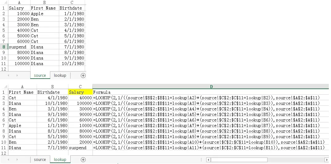
Let’s take a look at the formula at D2

=LOOKUP(2,1/((source!$B$2:$B$11=lookup!A2)*(source!$C$2:$C$11=lookup!B2)),{10000;20000;30000;...})

Parameter name	Parameter value
lookup_value	2
lookup_range	1/((source!$B$2:$B$11=lookup!A2)*(source!$C$2:$C$11=lookup!B2))
result_range	source!$A$2:$A$11

Below is the mechanism of the formula.

=LOOKUP(2,1/((source!$B$2:$B$11=lookup!A2)*(source!$C$2:$C$11=lookup!B2)),source!$A$2:$A$11)
=LOOKUP(2,1/({Apple;Ben;Ben;Cat;...="Cat"}*{29221;29222;29223;29224;...=29224}),{10000;20000;30000;40000;...})
=LOOKUP(2,1/({FALSE;FALSE;FALSE;TRUE;...}*{FALSE;FALSE;FALSE;TRUE;...}),{10000;20000;30000;40000;...})
=LOOKUP(2,1/{0;0;0;1;...},{10000;20000;30000;40000;...})
=LOOKUP(2,{#DIV/0;#DIV/0;#DIV/0;1;...},{10000;20000;30000;40000;...})
=40000

In the second parameter
1/{0;0;0;1;…}
The reason for dividing an array by 1 is that we want to turn all “0” to non numerical value (i.e. error)

{#DIV/0;#DIV/0;#DIV/0;1;...}

Afterwards, we apply LOOKUP formula and use “2” as the lookup_value parameter, where “2” is a constant that can be applied to other formula. When we lookup a value (2) which cannot be found in the array (a combination of 1 and #DIV/0), the Function will match the largest value (1) in the lookup_range (1 and #DIV/0) that is less than or equal to the value (2). In fact, you can also use “1” as the lookup_value parameter assume that value 1 can be found in the array, the Function will return the last matched value as well. As a normal practice, people tend to use “2” as parameter.

References – ASCII value of text

Note the conversion of Dec and Char

Dec	Hex	Oct	Char	Description
0	0	000		null
1	1	001		start of heading
2	2	002		start of text
3	3	003		end of text
4	4	004		end of transmission
5	5	005		enquiry
6	6	006		acknowledge
7	7	007		bell
8	8	010		backspace
9	9	011		horizontal tab
10	A	012		new line
11	B	013		vertical tab
12	C	014		new page
13	D	015		carriage return
14	E	016		shift out
15	F	017		shift in
16	10	020		data link escape
17	11	021		device control 1
18	12	022		device control 2
19	13	023		device control 3
20	14	024		device control 4
21	15	025		negative acknowledge
22	16	026		synchronous idle
23	17	027		end of trans. block
24	18	030		cancel
25	19	031		end of medium
26	1A	032		substitute
27	1B	033		escape
28	1C	034		file separator
29	1D	035		group separator
30	1E	036		record separator
31	1F	037		unit separator
32	20	040		space
33	21	041	!
34	22	042	“
35	23	043	#
36	24	044	$
37	25	045	%
38	26	046	&
39	27	047	‘
40	28	050	(
41	29	051	)
42	2A	052	*
43	2B	053	+
44	2C	054	,
45	2D	055	–
46	2E	056	.
47	2F	057	/
48	30	060	0
49	31	061	1
50	32	062	2
51	33	063	3
52	34	064	4
53	35	065	5
54	36	066	6
55	37	067	7
56	38	070	8
57	39	071	9
58	3A	072	:
59	3B	073	;
60	3C	074	<
61	3D	075	=
62	3E	076	>
63	3F	077	?
64	40	100	@
65	41	101	A
66	42	102	B
67	43	103	C
68	44	104	D
69	45	105	E
70	46	106	F
71	47	107	G
72	48	110	H
73	49	111	I
74	4A	112	J
75	4B	113	K
76	4C	114	L
77	4D	115	M
78	4E	116	N
79	4F	117	O
80	50	120	P
81	51	121	Q
82	52	122	R
83	53	123	S
84	54	124	T
85	55	125	U
86	56	126	V
87	57	127	W
88	58	130	X
89	59	131	Y
90	5A	132	Z
91	5B	133	[
92	5C	134	\
93	5D	135	]
94	5E	136	^
95	5F	137	_
96	60	140	`
97	61	141	a
98	62	142	b
99	63	143	c
100	64	144	d
101	65	145	e
102	66	146	f
103	67	147	g
104	68	150	h
105	69	151	i
106	6A	152	j
107	6B	153	k
108	6C	154	l
109	6D	155	m
110	6E	156	n
111	6F	157	o
112	70	160	p
113	71	161	q
114	72	162	r
115	73	163	s
116	74	164	t
117	75	165	u
118	76	166	v
119	77	167	w
120	78	170	x
121	79	171	y
122	7A	172	z
123	7B	173	{
124	7C	174	\|
125	7D	175	}
126	7E	176	~
127	7F	177	DEL