Excel Pivot Table Distinct Count to count unique value

This Excel tutorial explains how to use distinct count in Pivot Table to count number of unique value in a column grouped by other fields.

In Excel 2013, there is a new aggregate function in Pivot Table called Distinct Count, which counts number of unique value in a column. For example, if a column contains employee names, you can use the distinct count function to count number of unique employee names in the column such as below.

In this tutorial, I am going to demonstrate how to do distinct count.

Example – distinct count number of unique employee names by department

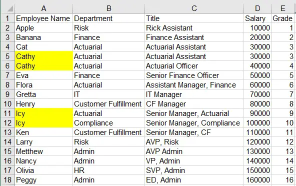
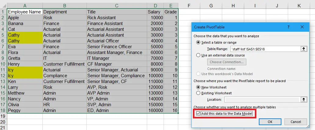
Suppose we have a staff list below. We want to see how many unique employee names are in the same department.


Select the concerned data, navigate to Insert > Pivot Table, then in the Create PivotTable dialog, check the box Add this data to the Data Model > OK

This option is very important as Distinct Count function will not be available if you don’t check this box.


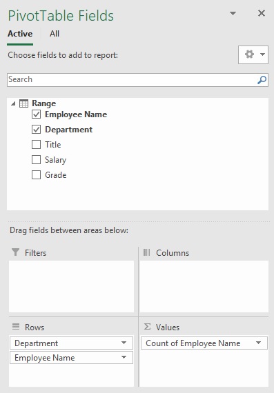
In the Pivot Table, drag Department and Employee Name to the Rows, drag Employee Name to the Values. By default, the aggregate function on the value is Count.


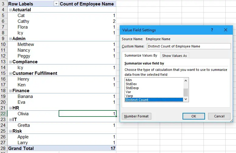
Click on the arrow next to Count of Employee Name, select Value Field Settings

In the Value Field Settings, select Distinct Count > OK


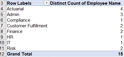
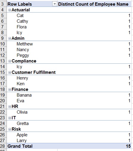
Now the Pivot Table displays the distinct count of employee name by department and display each all the names under each department.

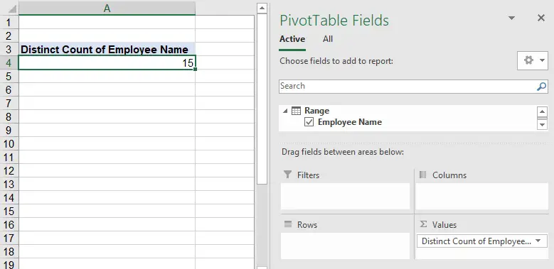
Overall, there are a total of 17 staff, as there are two Cathy and two Icy, the distinct count of employee name in the whole company is 15.


Alternatively, display the distinct count without displaying the employee name.


Outbound References

https://support.office.com/en-us/article/count-unique-values-among-duplicates-8d9a69b3-b867-490e-82e0-a929fbc1e273

Group Date and Ungroup Month in Excel Pivot Table

This Excel tutorial explains how to group dates and ungroup month in Excel Pivot Table to prevent auto grouping of Pivot Table in Excel 2016.

Group Date and Ungroup Month in Excel Pivot Table

Since Excel 2016,  when you drag a date field to a Pivot Table Pivot Table Row, the dates are  automatically grouped by months instead of showing each date. This is extremely annoying because  it is tricky to ungroup the months if it is the first time you encounter this issue.

In this post I am going to explain how to ungroup month in Excel Pivot Table and how to group dates by year or month.

Note that there is an Excel Option called Group dates in the AutoFilter Menu in Excel option, it does not work for Pivot Table Row Grouping. This option is for normal Auto Filter, not Pivot Table, so don’t get confused.

Ungroup Month in Excel Pivot Table

Suppose we have a data source which are dates from 2019 to 2021.


Insert a Pivot Table, and then drag the date field to Rows,the dates are automatically grouped by Year, Quarter and Month by default.

In order to display the original dates without grouping, right click on the data, select Group.

In the dates Grouping options, you can redefine how you want to group the dates. To display the original  dates on each row, highlight Days then OK.

Now the months are ungrouped and are displayed on each row.

Alternatively, you can simply right click on the date, then select Ungroup. this will ungroup every grouping.

Outbound References

https://support.office.com/en-gb/article/group-or-ungroup-data-in-a-pivottable-c9d1ddd0-6580-47d1-82bc-c84a5a340725