This SPSS Excel tutorial explains how to calculate One Way ANOVA in SPSS, Excel and manual calculation.
SPSS Excel One Way ANOVA
To determine if a sample comes from a population, we use one sample t test or Z Score.
To determine if two samples have the same mean, we use independent sample t test.
To determine if differences exist between two or more population means, we use One Way ANOVA (abbreviation of one way analysis of variance). The test statistics is called F test, it requires that the random variable be normally distributed with equal variances.
One Way ANOVA can be replaced by doing multiple t test, but the latter takes a lot more time. The main difference is that ANOVA has no direction, it only tells you whether there is a difference but it cannot tell whether one mean is larger than another.
One Way ANOVA – Semi-Manual calculation
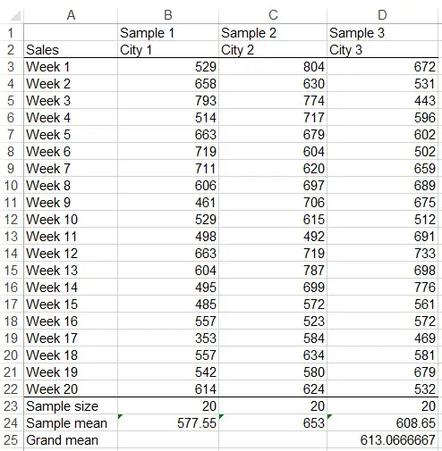
For example, we have collected 10 weekly sales data from the Supermarket A in three cities, we want to know if the mean sales are significantly different.
We create the below hypothesis:
Ho: μ1 = μ2 = μ3
H1: At least two means differ
Step 1: Sum of Squares for Treatments (SST) / Between treatments variation
In order to calculate the test statistics to see if the difference is significant, the first Step is to calculate the SST.
Calculate the sample mean for each sample and the grand mean of all data as below.
Then apply formula
SST = Summation of [sample n size * (sample n mean - grand mean)2]
In our example,
SST = 20(577.55-613.07)2 + 20(653-613.07)2 + 20(608.65-613.07)2
    = 57512.23
You can see from the formula that if sample mean is similar to grand mean, then SST should be closed to zero.
Step 2: Sum of Squares for Error (SSE)
After calculating SST, the next step is to calculate SSE, which is basically a sum of variance of all samples.
The first thing is to calculate the variance of each sample. To save time, use Excel Function VAR.S to calculate.
For example, sample variance of Sample 1 is
=VAR.S(B3:B22)
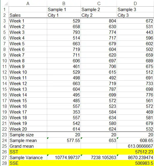
After getting the sample variance for each sample, apply formula
SSE = summation of [(sample size n - 1)* sample n variance]
In our example,
SSE = (20-1)*10774.99737 + (20-1)* 7238.105263 + (20-1)*8670.239474
    = 506983.5
Let’s summarize our results so far.
Step 3: Mean Square for Treatments (MST)
Degree of freedom for MST is number of treatments -1
MST = SST / (number of treatments -1)
Treatment in our example is 3 cities, therefore
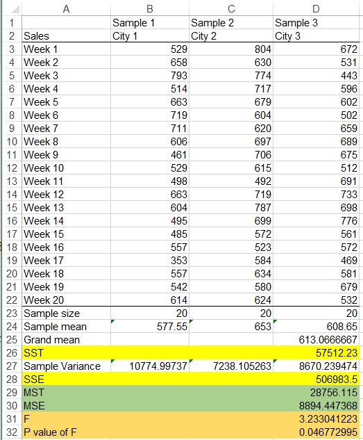
MST = 57512.23 / (3-1)
    = 28756.115
Step 4: Mean Square for Error (MSE)
Degree of freedom for MSE is number of sample data – number of treatments
MSE = SSE / (number of sample data - number of treatments)
In our example
MSE = 506983.5 / (60-3)
    = 8894.447368
Step 5: F Statistics and P value
F Statistics = MST / MSE
In our example
F Statistics = 8894.447368 / 28756.115
             = 3.233041223
To convert F Statistics into P value, we need the help of Excel Function F.DIST.RT
Syntax of F.DIST.RT
F.DIST.RT(x,deg_freedom1,deg_freedom2)
| X | Required. The value at which to evaluate the function. |
| Deg_freedom1 | Required. The numerator degrees of freedom. |
| Deg_freedom2 | Required. The denominator degrees of freedom. |
In our example, Deg_freedom1 is degree of freedom of MST, Deg_freedom1 is degree of freedom of MSE
P = F.DIST.RT( 3.233041223 ,2,57)
  = 0.046772995
Since P < 0.05, there is enough evidence to infer that the m ean weekly sales differ between the three cities.
One Way ANOVA – using Excel
Use the previous table.
In menu bar, navigate to Data > Data Analysis >Single Factor (if you don’t see Data Analysis, click here)
Select the Input Range as below

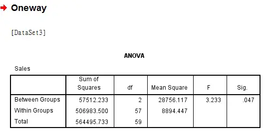
Now we get the same result

One Way ANOVA – using SPSS
Prepare a data set as below

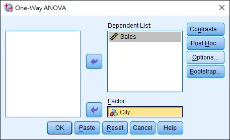
Analyze > Compare Means > One-Way ANOVA
Select Dependent List and Factor as below.
Now we have produced a similar table as Excel.