Excel VBA Import CSV into Excel using Workbooks.OpenText Method

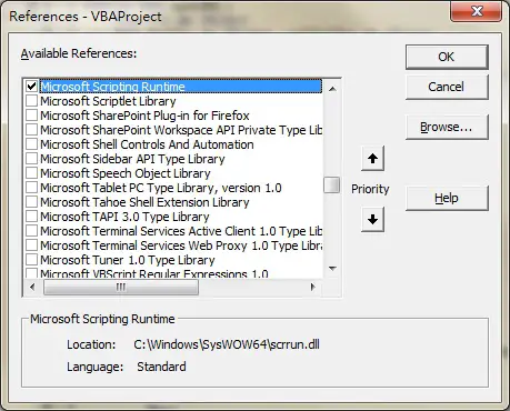
This Excel VBA tutorial explains how to import CSV into Excel automatically using Workbooks.OpenText Method. You may select different delimiters such as Tab, semicolon, comma, space.

You may also want to read:

Import Chinese CSV to Excel

Excel VBA convert CSV to Excel

Excel VBA Import CSV into Excel using Workbooks.OpenText Method

In Excel workbook, you can manually import a CSV file into Excel (Data > From Text / CSV). However, you have to select some options in advance such as delimiter. In order to import CSV into Excel automatically, you may use Workbooks.Open Text Method.

Syntax of Workbooks.Open Text Method

Workbooks.OpenText(FileName, Origin , StartRow , DataType , TextQualifier , ConsecutiveDelimiter , Tab , Semicolon , Comma , Space , Other , OtherChar , FieldInfo , TextVisualLayout , DecimalSeparator , ThousandsSeparator , TrailingMinusNumbers , Local)
NameRequired/OptionalData typeDescription
FileNameRequiredStringSpecifies the file name of the text file to be opened and parsed.
OriginOptionalVariantSpecifies the origin of the text file. Can be one of the following xlPlatform constants: xlMacintosh, xlWindows, or xlMSDOS. Additionally, this could be an integer representing the code page number of the desired code page. For example, “1256” would specify that the encoding of the source text file is Arabic (Windows). If this argument is omitted, the method uses the current setting of the File Origin option in the Text Import Wizard.
StartRowOptionalVariantThe row number at which to start parsing text. The default value is 1.
DataTypeOptionalVariantSpecifies the column format of the data in the file. Can be one of the following XlTextParsingType constants: xlDelimited or xlFixedWidth. If this argument is not specified, Microsoft Excel attempts to determine the column format when it opens the file.

NameValueDescription
xlDelimited1Default. Indicates that the file is delimited by delimiter characters.
xlFixedWidth2Indicates that the data in the file is arranged in columns of fixed widths.
TextQualifierOptionalVariant
NameValueDescription
xlTextQualifierDoubleQuote1Double quotation mark (“).
xlTextQualifierNone-4142No delimiter.
xlTextQualifierSingleQuote2Single quotation mark (‘).
ConsecutiveDelimiterOptionalVariantTrue to have consecutive delimiters considered one delimiter. The default is False.
TabOptionalVariantTrue to have the tab character be the delimiter (DataType must be xlDelimited). The default value is False.
SemicolonOptionalVariantTrue to have the semicolon character be the delimiter (DataType must be xlDelimited). The default value is False.
CommaOptionalVariantTrue to have the comma character be the delimiter (DataType must be xlDelimited). The default value is False.
SpaceOptionalVariantTrue to have the space character be the delimiter (DataType must be xlDelimited). The default value is False.
OtherOptionalVariantTrue to have the character specified by the OtherChar argument be the delimiter (DataType must be xlDelimited). The default value is False.
OtherCharOptionalVariant(required if Other is True). Specifies the delimiter character when Other is True. If more than one character is specified, only the first character of the string is used; the remaining characters are ignored.
FieldInfoOptionalVariantAn array containing parse information for individual columns of data. The interpretation depends on the value of DataType. When the data is delimited, this argument is an array of two-element arrays, with each two-element array specifying the conversion options for a particular column. The first element is the column number (1-based), and the second element is one of the XlColumnDataType constants specifying how the column is parsed.

NameValueDescription
xlDMYFormat4DMY date format.
xlDYMFormat7DYM date format.
xlEMDFormat10EMD date format.
xlGeneralFormat1General.
xlMDYFormat3MDY date format.
xlMYDFormat6MYD date format.
xlSkipColumn9Column is not parsed.
xlTextFormat2Text.
xlYDMFormat8YDM date format.
xlYMDFormat5YMD date format.
TextVisualLayoutOptionalVariantThe visual layout of the text.
DecimalSeparatorOptionalVariantThe decimal separator that Microsoft Excel uses when recognizing numbers. The default setting is the system setting.
ThousandsSeparatorOptionalVariantThe thousands separator that Excel uses when recognizing numbers. The default setting is the system setting.
TrailingMinusNumbersOptionalVariantSpecify True if numbers with a minus character at the end should be treated as negative numbers. If False or omitted, numbers with a minus character at the end are treated as text.
LocalOptionalVariantSpecify True if regional settings of the machine should be used for separators, numbers and data formatting.


Example – Import CSV into Excel using Workbooks.OpenText Method

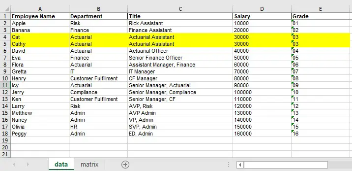
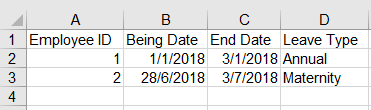
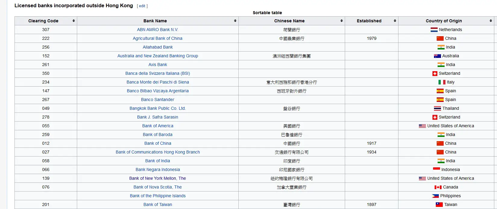
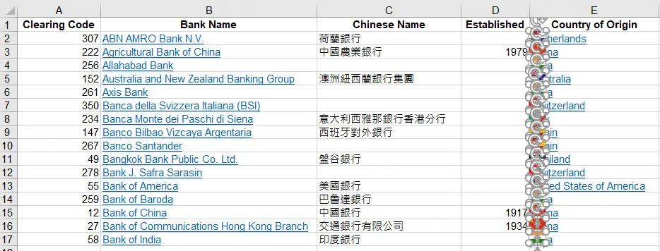
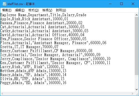
Suppose we have a staff list as below in csv file, in which the delimiter is comma with double quotation around text that contains comma (job title). Uur goal is import CSV into Excel and delimit the data automatically.

In the VBA code, for the case of a mix of double quotation and no double  quotation, we can skip the TextQualifier argument. We only have to identify the file path and delimiter as below.

Public Sub OpenCsvFile()
  .OpenText Filename:="C:\Users\WYMAN\Desktop\staff list.csv", DataType:=xlDelimited, comma:=True
 End Sub

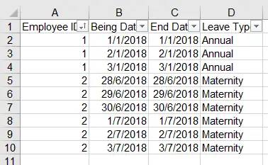
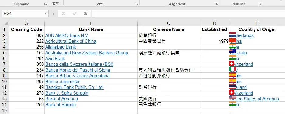
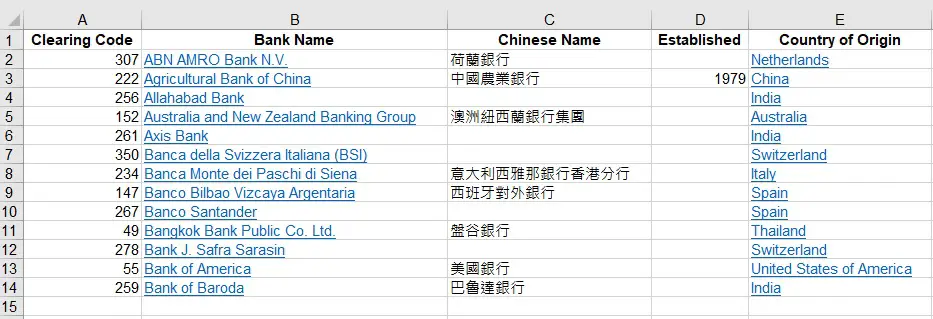
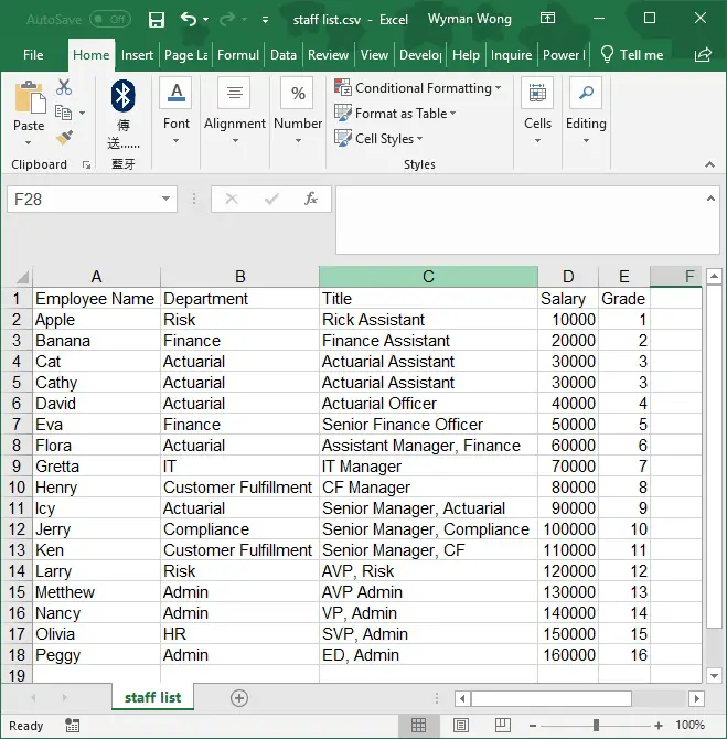
Create a new workbook, press ALT+F11 to insert the above procedure and then execute the procedure. The CSV file will open in Excel and the data is delimited properly.


Note that OpenText Method only opens the CSV in Excel but it is not importing the data into the current workbook.

To do so, we can add some codes to copy the worksheet over to the current workboook .

Public Sub OpenCsvFile()
    Application.ScreenUpdating = False  
    Workbooks.OpenText Filename:="C:\Users\WYMAN\Desktop\staff list.csv", DataType:=xlDelimited, comma:=True 
    With ActiveWorkbook
        .ActiveSheet.Copy After:=ThisWorkbook.Sheets(Sheets.Count)
        .Close
    End With   
    Cells.Select
    Cells.EntireColumn.AutoFit
    Range("A1").Select
    Application.ScreenUpdating = True
End Sub


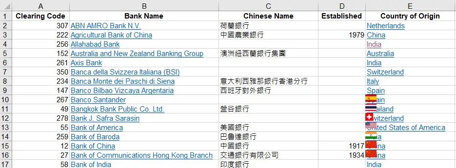
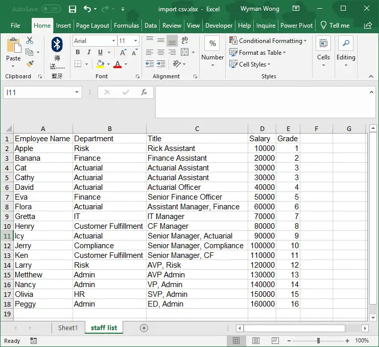
Execute the above procedure, now the delimited csv is added to the current workbook in a new worksheet.


Outbound References

https://docs.microsoft.com/zh-tw/office/vba/api/Excel.Workbooks.OpenText

Excel VBA Convert Text in Columns and Rows into Matrix Table

This Excel VBA tutorial explains how to convert text in columns and rows into Matrix Table. The Matrix table will display text instead of aggregated numbers.

You may also want to read:

Access Crosstab Query

Excel VBA Convert Text in Columns and Rows into Matrix Table

Using Excel Pivot Table, it is easy convert data into a Matrix Table with the help of Aggregate Functions such as Count, Sum, standard deviation. The information in the Matrix Table is displayed in aggregated numbers. Below is an example of a Matrix Table using aggregated function.

However if you want to create a Matrix Table in which you want to display nominal data (text) instead of aggregated numbers, Pivot Table is not technically possible.

In this tutorial, I am going demonstrate how to convert text in columns and rows into Matrix Table to display nominal data using Excel VBA.

VBA Code – Convert Columns and Rows into Matrix Table

Press ALT+F11 and insert the below VBA Procedure into a Module. Note that the you probably need to customize your own code in order to fit your needs, the below Procedure is just an example to show you how it can be done.

Public Sub convertMatrix()
    'assume data worksheet contains employee info, while matrix worksheet is the end result
    For r = 2 To Worksheets("data").Range("A" & Rows.Count).End(xlUp).Row
        Name = Worksheets("data").Range("A" & r)
        dept = Worksheets("data").Range("B" & r)
        
        Title = Worksheets("data").Range("C" & r)
        salary = Worksheets("data").Range("D" & r)
        grade = Worksheets("data").Range("E" & r)
    
        'search for department column number in the matrix table
        For c = 1 To Worksheets("matrix").Range("IV" & 1).End(xlToLeft).Column
            If Worksheets("matrix").Cells(1, c).Value = dept Then
                matrixCol = c
                Exit For
            End If
        Next c
        
        'search for grade row in the matrix table
        For g = 2 To Worksheets("matrix").Range("A" & Rows.Count).End(xlUp).Row
            If Worksheets("matrix").Cells(g, 1) = grade Then
                matrixRow = g
                Exit For
            End If
        Next g
        
        'Convert columns and rows into matrix table
        If Worksheets("matrix").Cells(g, c).Value <> "" Then
            Worksheets("matrix").Cells(g, c).Value = Worksheets("matrix").Cells(g, c).Value & vbCrLf & vbCrLf & Name & vbCrLf & Title & vbCrLf & salary
        Else
            Worksheets("matrix").Cells(g, c).Value = Name & vbCrLf & Title & vbCrLf & salary
        End If
    Next r
End Sub

Example – Convert Columns and Rows into Matrix Table

Suppose data worksheet contains the employee data that you want to convert into matrix table.

The employees highlighted in yellow are in the same department and of the same grade, I will demonstrate how it will display in the matrix table.


matrix worksheet contains the layout of the matrix, where we want to put the employee data into a matrix of Department and Grade.


Now execute the Procedure, employees and their info are put into the matrix table.

For employee Cat and Cathy, since they are in the same department and they are of the same grade, both their info are put into Cell B4, separated by a blank row.

Outbound References

https://support.office.com/en-us/article/Transpose-rotate-data-from-rows-to-columns-or-vice-versa-3419F2E3-BEAB-4318-AAE5-D0F862209744


Excel VBA search text in multiple Workbooks in folder

This Excel VBA tutorial explains how to search text in multiple Workbooks in a folder and subfolders, and display the result in a summary page, including which workbook, which worksheet, and which Cell contains the text.

You may also want to read:

Excel VBA INSTR Function

Excel loop workbooks in folders and subfolders with FSO

Excel VBA search text in multiple Workbooks in folder

Suppose you have multiple workbooks in a folder, and you want to know if any workbook contains a text you want to look for. The easiest way to do this is to press Ctrl + F in the folder you want to search for the text, then the search result will display.

However this method does not always work for different reasons. If it doesn’t work, then you need to look for an alternate approach. In this post, I will demonstrate how to use Excel VBA to search text in multiple workbooks in a folder and subfolders, and display the result in a summary page, including which workbook, which worksheet, and which Cell contains the text.

VBA Code – search text in multiple Workbooks in folder

Create a new workbook, press ALT+F11 and insert the below code in a Module. Do not save this workbook in the folder which you want to search the text.

Public Sub searchText()
    Dim FSO As Object
    Dim folder As Object, subfolder As Object
    Dim wb As Object
    Dim ws As Worksheet

    searchList = Array("orange", "apple", "pear")    'define the list of text you want to search, case insensitive
    
    Set FSO = CreateObject("Scripting.FileSystemObject")
    folderPath = "C:\test" 'define the path of the folder that contains the workbooks
    Set folder = FSO.GetFolder(folderPath)
    Dim thisWbWs, newWS As Worksheet
    
    'Create summary worksheet if not exist
    For Each thisWbWs In ActiveWorkbook.Worksheets
        If wsExists("summary") Then
            counter = 1
        End If
    Next thisWbWs
    
    If counter = 0 Then
        Set newWS = ThisWorkbook.Worksheets.Add(After:=Worksheets(Worksheets.Count))
        With newWS
            .Name = "summary"
            .Range("A1").Value = "Target Keyword"
            .Range("B1").Value = "Workbook"
            .Range("C1").Value = "Worksheet"
            .Range("D1").Value = "Address"
            .Range("E1").Value = "Cell Value"
        End With
    End If

    With Application
        .DisplayAlerts = False
        .ScreenUpdating = False
        .EnableEvents = False
        .AskToUpdateLinks = False
    End With
        
    'Check each workbook in main folder
    For Each wb In folder.Files
        If Right(wb.Name, 3) = "xls" Or Right(wb.Name, 4) = "xlsx" Or Right(wb.Name, 4) = "xlsm" Then
            Set masterWB = Workbooks.Open(wb)
            For Each ws In masterWB.Worksheets
              For Each Rng In ws.UsedRange
                For Each i In searchList
                    If InStr(1, Rng.Value, i, vbTextCompare) > 0 Then   'vbTextCompare means case insensitive. 
                        nextRow = ThisWorkbook.Sheets("summary").Range("A" & Rows.Count).End(xlUp).Row + 1
                        With ThisWorkbook.Sheets("summary")
                            .Range("A" & nextRow).Value = i
                            .Range("B" & nextRow).Value = Application.ActiveWorkbook.FullName
                            .Range("C" & nextRow).Value = ws.Name
                            .Range("D" & nextRow).Value = Rng.Address
                            .Range("E" & nextRow).Value = Rng.Value
                        End With
                    End If
                Next i
              Next Rng
            Next ws
            ActiveWorkbook.Close True
        End If
    Next
    
    'Check each workbook in sub folders
    For Each subfolder In folder.SubFolders
        For Each wb In subfolder.Files
            If Right(wb.Name, 3) = "xls" Or Right(wb.Name, 4) = "xlsx" Or Right(wb.Name, 4) = "xlsm" Then
                Set masterWB = Workbooks.Open(wb)
                For Each ws In masterWB.Worksheets
                  For Each Rng In ws.UsedRange
                    For Each i In searchList
                        If InStr(1, Rng.Value, i, vbTextCompare) > 0 Then
                            nextRow = ThisWorkbook.Sheets("summary").Range("A" & Rows.Count).End(xlUp).Row + 1
                            With ThisWorkbook.Sheets("summary")
                                .Range("A" & nextRow).Value = i
                                .Range("B" & nextRow).Value = Application.ActiveWorkbook.FullName
                                .Range("C" & nextRow).Value = ws.Name
                                .Range("D" & nextRow).Value = Rng.Address
                                .Range("E" & nextRow).Value = Rng.Value
                            End With
                        End If
                    Next i
                  Next Rng
                Next ws
                ActiveWorkbook.Close True
            End If
        Next
    Next
    With Application
        .DisplayAlerts = True
        .ScreenUpdating = True
        .EnableEvents = True
        .AskToUpdateLinks = True
    End With
    
    ThisWorkbook.Sheets("summary").Cells.Select
    ThisWorkbook.Sheets("summary").Cells.EntireColumn.AutoFit
    ThisWorkbook.Sheets("summary").Range("A1").Select
    
    
End Sub

Function wsExists(wksName As String) As Boolean 
    On Error Resume Next
    wsExists = CBool(Len(Worksheets(wksName).Name) > 0)
    On Error GoTo 0
End Function

Enable Microsoft Scripting Runtime

FileSystemObject (FSO) provides an API to access the Windows filesystem such as accessing Drive, TextStram, Folder, File.

You should be able to run FSO in Excel 2013. If you fail to run FSO Object, open VBE (ALT+F11) > Tools > References > Check the box Microsoft Scripting Runtine

loop_through_workbook

Example – search text in multiple Workbooks in folder

Suppose I want to search text “orange”, “apple”, “pear” in all workbooks under c:\test\, plus workbooks in one level down subfolders under c:\test\

I want to return search result even though the search text is a partial text in a Cell.

For example, if Cell A1 value of a workbook is “Orange Juice”, I still want to return the result because it contains “orange”.

Then create a new workbook that contains the VBA code, change the parameters that highlighted in red. Run the Procedure.

A summary worksheet is created, all the workbooks that contains “apple”, “orange” and “pear” will appear in the summary.


Excel VBA copy contents of protected worksheet

This Excel VBA tutorial explains how to copy contents of protected worksheet and then paste contents in another worksheet.

You may also want to read:

Excel VBA protect worksheet with password

Excel VBA hide worksheet with password (xlVeryHidden)

Copy contents of protected worksheet

Some authors would protect worksheets with password so that other people cannot modify and not even able to select the cells. I usually do it when I setup templates for users to fill in the data but I don’t want them to mess up my formula, so I protect my formula cells and allow them to modify other cells.

There is absolutely no way to modify the protected worksheet without knowing the password, and you cannot manually copy the contents because you are not allowed select the cells.

However, with the help of VBA, you can easily copy the contents and paste to another worksheet without clicking on the cells.

VBA Code – Copy contents of protected worksheet

Suppose you want to copy all contents and formats from a worksheet called “protected ws”, and then paste to a worksheet called “new ws”, then use the below VBA code.

Public Sub copyContents()
  Sheets("protected ws").Cells.Copy
  Sheets("new ws").Range("A1").Select
  ActiveSheet.Paste
End Sub

This VBA is very simple to use, just change the worksheet names. This VBA not only works for protected worksheet, but also work for normal worksheet if you want to copy contents.

VBA Code – Copy protected workbook

The below VBA copy and whole protected workbook and save as a new workbook under the current workbook path.

Sub cpyWB()
    Application.ScreenUpdating = False
    Application.DisplayAlerts = False
     
    Set newbook = Workbooks.Add
    defaultSheet = newbook.Sheets.Count
     
    For Each WS In ThisWorkbook.Sheets
        Set newWS = Sheets.Add(After:=Sheets(newbook.Sheets.Count))
        newWS.Name = WS.Name
        ThisWorkbook.Sheets(WS.Name).Cells.Copy
        newbook.Sheets(WS.Name).Paste
    Next WS
    
    For i = 1 To defaultSheet
        newbook.Sheets("Sheet" & i).Delete
    Next i

    newbook.SaveAs ThisWorkbook.Path & "\Copy - " & ThisWorkbook.Name
    newbook.Close
    Application.DisplayAlerts = True
    Application.ScreenUpdating = True
End Sub


Excel VBA convert date period to date row

This Excel VBA tutorial explains how to convert date period to date row.

Excel VBA convert date period into date row

Different systems store date transactions differently. For example, if you apply for annual leave from Jan 1 to Jan 3, some system store the data in data base using date period

Begin DateEnd Date
1/1/20181/3/2018

However some system store one date per row.

Begin DateEnd Date
1/1/20181/1/2018
2/1/20182/1/2018
3/1/20181/3/2018

To convert from one format to another is extremely difficult and time consuming. In this tutorial, I will demonstrate how to convert date period to date row, because I personally think this data structure is easier to handle.

VBA code – convert date period to date row

Press ALT+F11, insert the code into a Module.

Public Sub convertDate()
  beginDtCol = "B"  'column that contains begin date period
  endDtCol = "C"   'column that contains end date period
  For r = Range(beginDtCol & Rows.Count).End(xlUp).Row To 2 Step -1
    If Range(endDtCol & r) - Range(beginDtCol & r) > 0 Then
      For i = 1 To Range(endDtCol & r) - Range(beginDtCol & r)
        Rows(r).EntireRow.Copy
        Range("A" & Range(beginDtCol & Rows.Count).End(xlUp).Row + 1).Select
        ActiveSheet.Paste
 
        Range(beginDtCol & Range(beginDtCol & Rows.Count).End(xlUp).Row) = Range(beginDtCol & r) + i
        Range(endDtCol & Range(endDtCol & Rows.Count).End(xlUp).Row) = Range(beginDtCol & r) + i
      Next i
      Range(endDtCol & r) = Range(beginDtCol & r)
    End If
  Next
  Range("A1").AutoFilter
  'sort column A
  ActiveSheet.AutoFilter.Sort.SortFields.Add Key:=Range("A:A"), SortOn:=xlSortOnValues, Order:=xlAscending, DataOption:=xlSortNormal
  ActiveSheet.AutoFilter.Sort.Apply
End Su


Example – convert date period to date row

Suppose we have two leave transactions below.


Run the Macro, date period is converted to date row. In addition, all the other column values are copied.

Column A is also sorted in ascending order. Change the code at the bottom if you want to sort another column.


Excel VBA filter value then copy filtered data to new worksheet

This Excel VBA tutorial explains how to automate AutoFilter to filter value and then copy data to new worksheet or copy data to new workbook.

You may also want to read:

Excel VBA copy each worksheet to new workbook

Access VBA auto generate mass report by group to Excel

Filter value then copy filtered data to new worksheet

I find it very difficult to come up with a suitable title and key words for this post. I will try to describe what this Macro does with an example.

Suppose you have a staff list as below.

Now you want to create one worksheet for each department.

Worksheet “HR”

DepartmentStaff IDName
HR1Peter
HR2Apple
HR3Banana

Worksheet “IT”

DepartmentStaff IDName
IT2John
IT6Judy

Worksheet “CS”

DepartmentStaff IDName
CS4Cat
CS5David

If you have a hundred of unique department, it will take you forever to manually copy the data over to the new worksheet. What I want to achieve is to create a Macro to automatically filter each department and then copy the contents to a new worksheet.

VBA Code – Filter value then copy filtered data to new worksheet

To use this Macro:

1) Copy and paste the below code in a Module

2) Modify the 3rd row of code where the targetCol is the column that contains the department you want to break into separate worksheets

3) Select the worksheet that contains the staff list

4) Run the Macro

Public Sub FilterThenCopy()
   Dim ws, newWS, currentWS As Worksheet
   targetCol = 1   'define which column you want to break
   Dim objDict As Variant
   Set objDict = CreateObject("Scripting.Dictionary")
   Set currentWS = ActiveSheet
   'Add unique value in targetCol to the dictionary
   Application.DisplayAlerts = False
   For r = 2 To Cells(Rows.Count, targetCol).End(xlUp).Row
     If Not objDict.exists(Cells(r, targetCol).Value) Then
       objDict.Add Cells(r, targetCol).Value, Cells(r, targetCol).Value
     End If
   Next r

  If currentWS.AutoFilterMode = True Then
     currentWS.UsedRange.AutoFilter
  End If
  currentWS.UsedRange.AutoFilter
  For Each k In objDict.Keys
    currentWS.UsedRange.AutoFilter field:=targetCol, Criteria1:=objDict.Item(k)
   'delete worksheet if worksheet of item(k) exist
    For Each ws In ActiveWorkbook.Worksheets
      If wsExists(objDict.Item(k)) Then
        Sheets(objDict.Item(k)).Delete
      End If
    Next ws
   'crate worksheet using item(k) name
    Set newWS = ThisWorkbook.Worksheets.Add(After:=Worksheets(Worksheets.Count))
    newWS.Name = objDict.Item(k)
    'copy filtered contents to new worksheet
    currentWS.UsedRange.SpecialCells(xlCellTypeVisible).Copy
    newWS.Range("A1").Select
    newWS.Paste
  Next k
  currentWS.Activate
  currentWS.AutoFilterMode = False
  Application.DisplayAlerts = True
End Sub

Function wsExists(wksName As String) As Boolean
   On Error Resume Next
   wsExists = CBool(Len(Worksheets(wksName).Name) > 0)
   On Error GoTo 0
End Function

Result

After you run the Macro, 3 new worksheets are created. The format should also be copied from the master staff list.

Filter value then copy to new workbook

Instead of copying data to new worksheet, you may want to copy to new workbook. Previously I wrote a post about copying each worksheet to new workbook, you just need to run the above Macro, and then run the copy to new workbook Macro. Click here to read my previous post.

Use Microsoft Access to generate mass report by Group

If you want to achieve the same result using Microsoft Access, click here to read my previous post. The advantage of using Microsoft Access is that you can use Query to transform data before export.

Access Excel VBA sort Array items

This Access Excel VBA tutorial explains how to sort Array items in VBA in ascending order / descending order.

You may also want to read:

Use VBA Excel Function to sort data in ascending order

Access Excel VBA sort Array items

In an Array, you may have stored items that you want to sort. For example, if you store a name list, you may want to sort them in alphabetical order (Apple, Banana, Cat…).  If you store a number list, you may want to sort them in ascending order (100, 200, 400, 700…). Since there is no built in VBA function to sort Array items, we have to write a sorting logic manually to do the job. In this post, I write a Procedure that uses Bubble Sort method to do the sorting.

After sorting the Array items, you may want to know the ranking (Index) of specific Array items. Read my previous post to learn more.

Sort Array items in ascending order

The sorting sequence is:  blank > symbol > number > alphabet (disregard capital letter or not)

VBA Code

Public Sub sortAscending(arr as variant)
  Dim arr As Variant
  arr = Array(30, 70, 50, 99)
  lngMin = LBound(arr)
  lngMax = UBound(arr)
  For i = lngMin To lngMax - 1
    For j = i + 1 To lngMax
      If arr(i) > arr(j) Then
        strTemp = arr(i)
        arr(i) = arr(j)
        arr(j) = strTemp
      End If
    Next j
  Next i
End Sub

Example

Public Sub test()
   Dim arr As Variant
   arr = Array(30, 70, 50, 99)
   Call sortAscending(arr)
   MsgBox (arr(0) & " " & arr(1) & " " & arr(2) & " " & arr(3))
End Sub

Public Sub sortAscending(arr As Variant)
   lngMin = LBound(arr)
   lngMax = UBound(arr)
   For i = lngMin To lngMax - 1
     For j = i + 1 To lngMax
       If arr(i) > arr(j) Then
         strTemp = arr(i)
         arr(i) = arr(j)
         arr(j) = strTemp
       End If
     Next j
   Next i
End Sub

Result


Sort Array items in descending order

Simply replace  arr(i) > arr(j) with  arr(i) < arr(j) to sort Array in descending order.

Public Sub sortDescending(arr As Variant)
  lngMin = LBound(arr)
  lngMax = UBound(arr)
  For i = lngMin To lngMax - 1
    For j = i + 1 To lngMax
      If arr(i) < arr(j) Then
        strTemp = arr(i)
        arr(i) = arr(j)
        arr(j) = strTemp
      End If
    Next j
  Next i
End Sub


Excel convert data from column to row

This Excel VBA tutorial explains how to convert data from column to row (transform one column data to one row).

You may also want to read:

Excel VBA consolidate multiple workbooks into one workbook

Excel VBA combine worksheets columns into one worksheet

Excel convert data from column to row

Different database have different structure. Some database put similar data in the same column with different rows, while some database put data in different columns. .Let’s take an example.

Type 1: all payment types are arranged in the same column

Employee IDPayment TypeAmount
1Salary10000
1Allowance1000
2Salary10000
3Salary10000
4Salary10000

Type 2: each column for each payment type

Employee IDSalaryAllowance
1100001000
210000
310000
410000

In this tutorial, I will demonstrate how to use VBA to convert data from column to row (from type 2 to type 1).

VBA Code – convert data from column to row

Please note that when I wrote this Macro, I only tested the scenarios in my below examples. For any other exceptional scenarios that I am not aware, my Macro may not function probably (I don’t know what I don’t know).

Press ALT+F11 and then paste the below code in a new Module

Public Sub convert()
    'the column data that you want to repeat (such as name) as you move the data down the row
    ReptColSt = "A"
    ReptColEd = "C"
    'column that contains the data that you want to move down the row. This includes the first column that acts as the header for other moved data
    dataColSt = "D"
    dataColEd = "I"
    'the number of columns the you want to move as a set to a single row
    noOfDataCol = 1  

    colLastRow = ActiveSheet.Range("A" & Rows.Count).End(xlUp).Row
    ReptColStNum = Range(ReptColSt & 1).Column
    ReptColEdNum = Range(ReptColEd & 1).Column
    noOfReptCol = ReptColEdNum - ReptColStNum + 1
    dataColStNum = Range(dataColSt & 1).Column
    dataColEdNum = Range(dataColEd & 1).Column
    lastRow = ActiveSheet.Range("A" & Rows.Count).End(xlUp).Row

    For r = 2 To colLastRow
        For c = dataColStNum To dataColEdNum
            If c = dataColStNum Then
                    For k = 2 To lastRow
                        Cells(1, dataColStNum).Copy Cells(k, dataColEdNum + 1)
                    Next
            ElseIf (c - dataColStNum - noOfDataCol) Mod noOfDataCol = 0 Then
                    nextRow = ActiveSheet.Range("A" & Rows.Count).End(xlUp).Row + 1
                    Range(ReptColSt & r & ":" & ReptColEd & r).Copy Range(ReptColSt & nextRow)
                    Cells(1, c).Copy Cells(nextRow, dataColEdNum + 1)
                    For n = 0 To noOfDataCol - 1
                        Cells(r, c + n).Copy Cells(nextRow, dataColStNum + n)
                    Next
            End If
        Next c
    Next r
    Cells(1, dataColEdNum + 1).Value = "Original Column"
    'to delete the original data columns
    Range(Cells(1, dataColStNum + noOfDataCol), Cells(1, dataColEdNum)).EntireColumn.Delete  
    'to delete rows with empty records
    lastRow = ActiveSheet.Range("A" & Rows.Count).End(xlUp).Row
    For m = lastRow To 2 Step -1
        counter = 0
        For n = dataColStNum To dataColStNum + noOfDataCol - 1
            If Cells(m, n).Value = "" Then
                counter = counter + 1
            End If
            If counter = noOfDataCol Then
                Rows(m).EntireRow.Delete
            End If
        Next n
     Next m
End Sub

Convert all columns to a single column

A little explanation for this code with an example. In the below Table, my goal is to move each salary and bonus column from column D to I to the same column (column D). For each newly added row, I want column A to C to repeat.

In the parameter line of code, I need to set the followings

 'the column data that you want to repeat (such as name) as you move the data down the row
 ReptColSt = "A"
 ReptColEd = "C"
 'column that contains the data that you want to move down the row. This includes the first column that acts as the header for other moved data
 dataColSt = "D"
 dataColEd = "I"
 'the number of columns the you want to move as a set to a single row
 noOfDataCol = 1

Run the Macro and get the below result.

Column E is a new column created to indicate which column the data in column D originally came from. Column D header has to be manually change as it is the original header before conversion, so it is more appropriate to change it to “Amount”.

Convert all columns to a multiple columns

Suppose I want to convert all data columns to fit into column D (Salary) and column E (Bonus). Use the same Macro as above but update the below parameter to 2.

 'the number of columns the you want to move as a set to a single row
 noOfDataCol = 2

Run the Macro and get the below result.

Similar to the above example, column F is the new column to indicate where column D and E data originally came from. Column D and E headers should be renamed appropriately, such as “Salary” and “Bonus”.


Excel delete all pictures or delete all pictures in specific Cells

This Excel tutorial explains how to delete all pictures in a worksheet or delete all pictures in specific Cells.

Excel delete all pictures

When you copy contents from website to Excel, it is unavoidable to also copy unwanted pictures. As some websites contains dozens of pictures, it is a waste of time to delete pictures one by one. In this tutorial, I will demonstrate how to  delete all pictures at once.

Let’s say I want to copy the below table from a website. In the Country of Origin field, each country has a logo of the country.


When we copy the table to Excel, the country logos are also copied.


Press F5 > Special > Objects > OK

Now all the pictures are selected, click on keyboard Delete button to delete all pictures.

Excel VBA delete all pictures

Press ALT+F11, insert the below code in a Module

Public Sub delete_picture()
 For Each shp In ActiveSheet.Shapes
 shp.Delete
 Next
End Sub

Run the Macro, now all the pictures are deleted.

Alternatively, you can use DrawingObjects.Delete

Sub delete_picture2()
 ActiveSheet.DrawingObjects.Delete
End Sub

As you can notice in the VBA code, DrawingObjects have Delete Method, but not Shapes. If you want to use For Loop to loop through each object, you have to use Shapes.

Excel VBA delete all pictures in specific Cells

I haven’t found a way to delete pictures in specific Cells without using VBA, so I believe VBA is the way to go.

Lets say we want to delete pictures in specific Cells, only pictures in Range E2:E9.

Use TopLeftCell Property to determine if a Cell contains a picture. Click here to learn more about the Intersect Method.

Public Sub delete_picture()
 For Each shp In ActiveSheet.Shapes
 If Not Intersect(shp.TopLeftCell, [E2:E9]) Is Nothing Then shp.Delete
 Next
End Sub

Run the Macro to get the below result


Excel VBA unmerge columns automatically

This Excel VBA tutorial explains how to unmerge columns automatically and then delete blank column.

You may also want to read:

Excel VBA reformat merged cells to row

Excel VBA separate line break data into different rows

Excel VBA unmerge columns automatically

For some systems, when you export a non-Excel report (e.g. PDF) to Excel format, some columns could be merged in order to fit the width of the original report layout. Even for Sharepoint, this formatting issue also happens.

In order to address this issue, I have created a Macro to unmerge those merged columns.

VBA Code -unmerge columns automatically

Press ALT+F11, copy and paste the below Procedures to a new Module.

Public Sub unmerge()
    If ActiveSheet.UsedRange.SpecialCells(xlCellTypeLastCell).MergeCells = True Then
        ActiveSheet.UsedRange.SpecialCells(xlCellTypeLastCell).unmerge
    End If
    
    usedRangeLastColNum = ActiveSheet.UsedRange.SpecialCells(xlCellTypeLastCell).Column

    For c = usedRangeLastColNum To 1 Step -1
        If Cells(1, c).Value = "" Then
            Columns(c).EntireColumn.Delete
        End If
    Next
End Sub

Explanation:

This Macro loops through the row 1 of right column to left column. If the Cell value is blanked, then delete the whole column.

Take field C as example.

Cell C1, D1 and E1 are merged. For merged cells, the Cell value lies in the first Cell on the left. Therefore C1 value is “Field C”, but D1 and E1 are blank.

When looping through range E1 to C1, column D and E are deleted because they contain blank value, leaving only column C.

For column G to J is a little tricky. The last used cell is G12, not J12, so I cannot delete column H to J.  As a workaround, I check whether column H12 is merged, then unmerge it so that I can loop from J1.

Example -unmerge columns automatically

Run the Macro to get the below result.