Excel Pivot Table Distinct Count to count unique value

This Excel tutorial explains how to use distinct count in Pivot Table to count number of unique value in a column grouped by other fields.

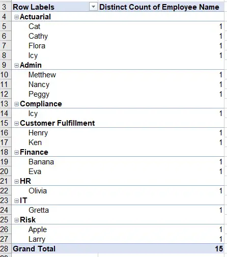
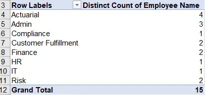
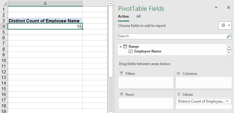
In Excel 2013, there is a new aggregate function in Pivot Table called Distinct Count, which counts number of unique value in a column. For example, if a column contains employee names, you can use the distinct count function to count number of unique employee names in the column such as below.

In this tutorial, I am going to demonstrate how to do distinct count.

Example – distinct count number of unique employee names by department

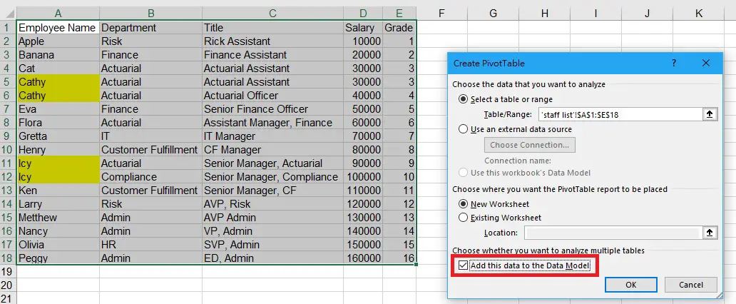
Suppose we have a staff list below. We want to see how many unique employee names are in the same department.


Select the concerned data, navigate to Insert > Pivot Table, then in the Create PivotTable dialog, check the box Add this data to the Data Model > OK

This option is very important as Distinct Count function will not be available if you don’t check this box.


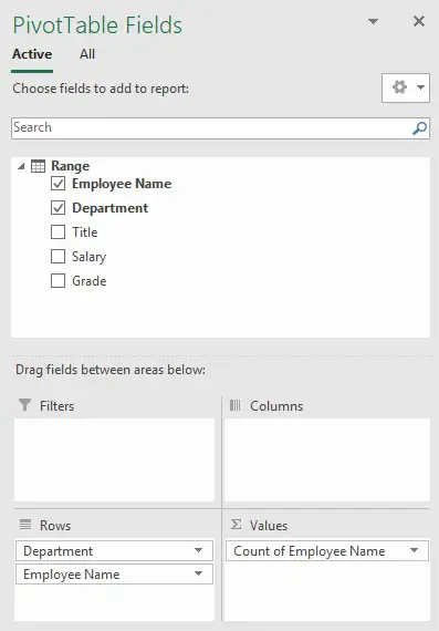
In the Pivot Table, drag Department and Employee Name to the Rows, drag Employee Name to the Values. By default, the aggregate function on the value is Count.


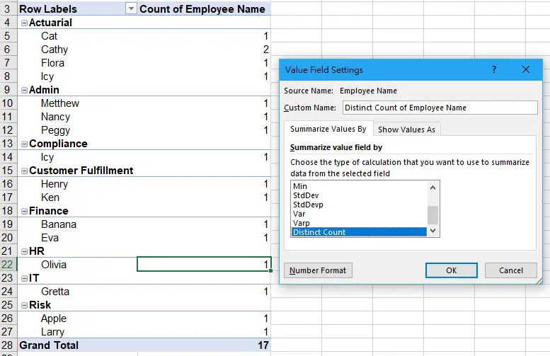
Click on the arrow next to Count of Employee Name, select Value Field Settings

In the Value Field Settings, select Distinct Count > OK


Now the Pivot Table displays the distinct count of employee name by department and display each all the names under each department.

Overall, there are a total of 17 staff, as there are two Cathy and two Icy, the distinct count of employee name in the whole company is 15.


Alternatively, display the distinct count without displaying the employee name.


Outbound References

https://support.office.com/en-us/article/count-unique-values-among-duplicates-8d9a69b3-b867-490e-82e0-a929fbc1e273

Excel VBA Import CSV into Excel using Workbooks.OpenText Method

This Excel VBA tutorial explains how to import CSV into Excel automatically using Workbooks.OpenText Method. You may select different delimiters such as Tab, semicolon, comma, space.

You may also want to read:

Import Chinese CSV to Excel

Excel VBA convert CSV to Excel

Excel VBA Import CSV into Excel using Workbooks.OpenText Method

In Excel workbook, you can manually import a CSV file into Excel (Data > From Text / CSV). However, you have to select some options in advance such as delimiter. In order to import CSV into Excel automatically, you may use Workbooks.Open Text Method.

Syntax of Workbooks.Open Text Method

Workbooks.OpenText(FileName, Origin , StartRow , DataType , TextQualifier , ConsecutiveDelimiter , Tab , Semicolon , Comma , Space , Other , OtherChar , FieldInfo , TextVisualLayout , DecimalSeparator , ThousandsSeparator , TrailingMinusNumbers , Local)
NameRequired/OptionalData typeDescription
FileNameRequiredStringSpecifies the file name of the text file to be opened and parsed.
OriginOptionalVariantSpecifies the origin of the text file. Can be one of the following xlPlatform constants: xlMacintosh, xlWindows, or xlMSDOS. Additionally, this could be an integer representing the code page number of the desired code page. For example, “1256” would specify that the encoding of the source text file is Arabic (Windows). If this argument is omitted, the method uses the current setting of the File Origin option in the Text Import Wizard.
StartRowOptionalVariantThe row number at which to start parsing text. The default value is 1.
DataTypeOptionalVariantSpecifies the column format of the data in the file. Can be one of the following XlTextParsingType constants: xlDelimited or xlFixedWidth. If this argument is not specified, Microsoft Excel attempts to determine the column format when it opens the file.

NameValueDescription
xlDelimited1Default. Indicates that the file is delimited by delimiter characters.
xlFixedWidth2Indicates that the data in the file is arranged in columns of fixed widths.
TextQualifierOptionalVariant
NameValueDescription
xlTextQualifierDoubleQuote1Double quotation mark (“).
xlTextQualifierNone-4142No delimiter.
xlTextQualifierSingleQuote2Single quotation mark (‘).
ConsecutiveDelimiterOptionalVariantTrue to have consecutive delimiters considered one delimiter. The default is False.
TabOptionalVariantTrue to have the tab character be the delimiter (DataType must be xlDelimited). The default value is False.
SemicolonOptionalVariantTrue to have the semicolon character be the delimiter (DataType must be xlDelimited). The default value is False.
CommaOptionalVariantTrue to have the comma character be the delimiter (DataType must be xlDelimited). The default value is False.
SpaceOptionalVariantTrue to have the space character be the delimiter (DataType must be xlDelimited). The default value is False.
OtherOptionalVariantTrue to have the character specified by the OtherChar argument be the delimiter (DataType must be xlDelimited). The default value is False.
OtherCharOptionalVariant(required if Other is True). Specifies the delimiter character when Other is True. If more than one character is specified, only the first character of the string is used; the remaining characters are ignored.
FieldInfoOptionalVariantAn array containing parse information for individual columns of data. The interpretation depends on the value of DataType. When the data is delimited, this argument is an array of two-element arrays, with each two-element array specifying the conversion options for a particular column. The first element is the column number (1-based), and the second element is one of the XlColumnDataType constants specifying how the column is parsed.

NameValueDescription
xlDMYFormat4DMY date format.
xlDYMFormat7DYM date format.
xlEMDFormat10EMD date format.
xlGeneralFormat1General.
xlMDYFormat3MDY date format.
xlMYDFormat6MYD date format.
xlSkipColumn9Column is not parsed.
xlTextFormat2Text.
xlYDMFormat8YDM date format.
xlYMDFormat5YMD date format.
TextVisualLayoutOptionalVariantThe visual layout of the text.
DecimalSeparatorOptionalVariantThe decimal separator that Microsoft Excel uses when recognizing numbers. The default setting is the system setting.
ThousandsSeparatorOptionalVariantThe thousands separator that Excel uses when recognizing numbers. The default setting is the system setting.
TrailingMinusNumbersOptionalVariantSpecify True if numbers with a minus character at the end should be treated as negative numbers. If False or omitted, numbers with a minus character at the end are treated as text.
LocalOptionalVariantSpecify True if regional settings of the machine should be used for separators, numbers and data formatting.


Example – Import CSV into Excel using Workbooks.OpenText Method

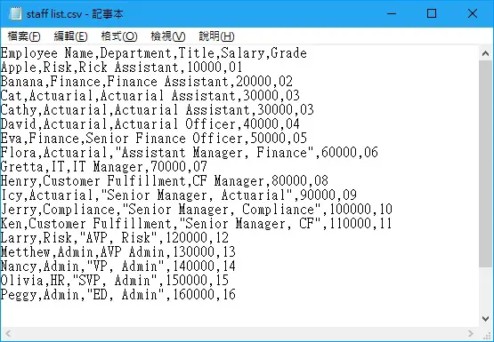
Suppose we have a staff list as below in csv file, in which the delimiter is comma with double quotation around text that contains comma (job title). Uur goal is import CSV into Excel and delimit the data automatically.

In the VBA code, for the case of a mix of double quotation and no double  quotation, we can skip the TextQualifier argument. We only have to identify the file path and delimiter as below.

Public Sub OpenCsvFile()
  .OpenText Filename:="C:\Users\WYMAN\Desktop\staff list.csv", DataType:=xlDelimited, comma:=True
 End Sub

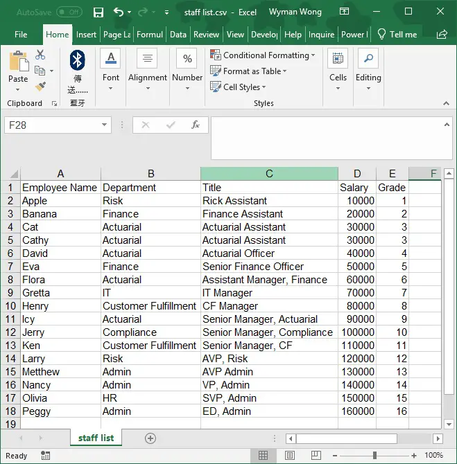
Create a new workbook, press ALT+F11 to insert the above procedure and then execute the procedure. The CSV file will open in Excel and the data is delimited properly.


Note that OpenText Method only opens the CSV in Excel but it is not importing the data into the current workbook.

To do so, we can add some codes to copy the worksheet over to the current workboook .

Public Sub OpenCsvFile()
    Application.ScreenUpdating = False  
    Workbooks.OpenText Filename:="C:\Users\WYMAN\Desktop\staff list.csv", DataType:=xlDelimited, comma:=True 
    With ActiveWorkbook
        .ActiveSheet.Copy After:=ThisWorkbook.Sheets(Sheets.Count)
        .Close
    End With   
    Cells.Select
    Cells.EntireColumn.AutoFit
    Range("A1").Select
    Application.ScreenUpdating = True
End Sub


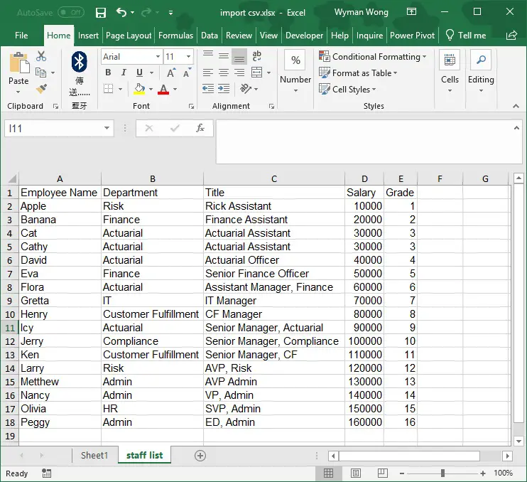
Execute the above procedure, now the delimited csv is added to the current workbook in a new worksheet.


Outbound References

https://docs.microsoft.com/zh-tw/office/vba/api/Excel.Workbooks.OpenText

Excel VBA Convert Text in Columns and Rows into Matrix Table

This Excel VBA tutorial explains how to convert text in columns and rows into Matrix Table. The Matrix table will display text instead of aggregated numbers.

You may also want to read:

Access Crosstab Query

Excel VBA Convert Text in Columns and Rows into Matrix Table

Using Excel Pivot Table, it is easy convert data into a Matrix Table with the help of Aggregate Functions such as Count, Sum, standard deviation. The information in the Matrix Table is displayed in aggregated numbers. Below is an example of a Matrix Table using aggregated function.

However if you want to create a Matrix Table in which you want to display nominal data (text) instead of aggregated numbers, Pivot Table is not technically possible.

In this tutorial, I am going demonstrate how to convert text in columns and rows into Matrix Table to display nominal data using Excel VBA.

VBA Code – Convert Columns and Rows into Matrix Table

Press ALT+F11 and insert the below VBA Procedure into a Module. Note that the you probably need to customize your own code in order to fit your needs, the below Procedure is just an example to show you how it can be done.

Public Sub convertMatrix()
    'assume data worksheet contains employee info, while matrix worksheet is the end result
    For r = 2 To Worksheets("data").Range("A" & Rows.Count).End(xlUp).Row
        Name = Worksheets("data").Range("A" & r)
        dept = Worksheets("data").Range("B" & r)
        
        Title = Worksheets("data").Range("C" & r)
        salary = Worksheets("data").Range("D" & r)
        grade = Worksheets("data").Range("E" & r)
    
        'search for department column number in the matrix table
        For c = 1 To Worksheets("matrix").Range("IV" & 1).End(xlToLeft).Column
            If Worksheets("matrix").Cells(1, c).Value = dept Then
                matrixCol = c
                Exit For
            End If
        Next c
        
        'search for grade row in the matrix table
        For g = 2 To Worksheets("matrix").Range("A" & Rows.Count).End(xlUp).Row
            If Worksheets("matrix").Cells(g, 1) = grade Then
                matrixRow = g
                Exit For
            End If
        Next g
        
        'Convert columns and rows into matrix table
        If Worksheets("matrix").Cells(g, c).Value <> "" Then
            Worksheets("matrix").Cells(g, c).Value = Worksheets("matrix").Cells(g, c).Value & vbCrLf & vbCrLf & Name & vbCrLf & Title & vbCrLf & salary
        Else
            Worksheets("matrix").Cells(g, c).Value = Name & vbCrLf & Title & vbCrLf & salary
        End If
    Next r
End Sub

Example – Convert Columns and Rows into Matrix Table

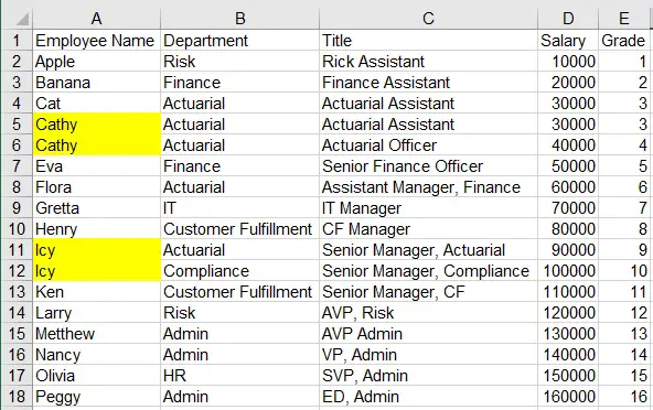
Suppose data worksheet contains the employee data that you want to convert into matrix table.

The employees highlighted in yellow are in the same department and of the same grade, I will demonstrate how it will display in the matrix table.


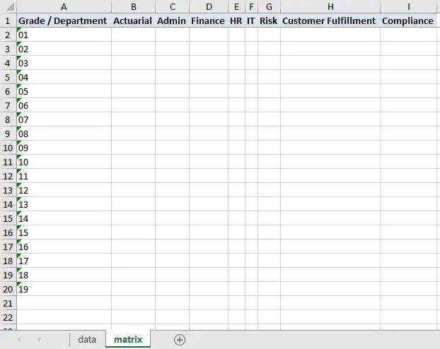
matrix worksheet contains the layout of the matrix, where we want to put the employee data into a matrix of Department and Grade.


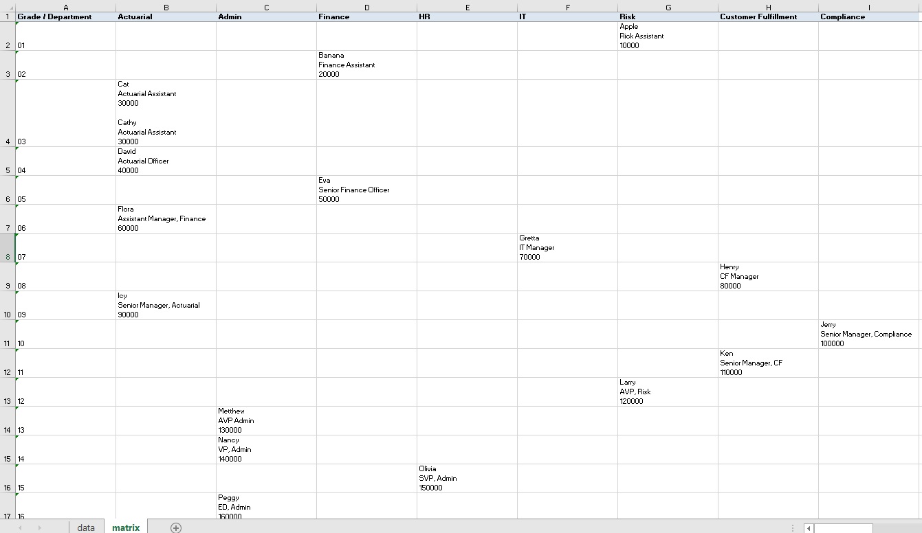
Now execute the Procedure, employees and their info are put into the matrix table.

For employee Cat and Cathy, since they are in the same department and they are of the same grade, both their info are put into Cell B4, separated by a blank row.

Outbound References

https://support.office.com/en-us/article/Transpose-rotate-data-from-rows-to-columns-or-vice-versa-3419F2E3-BEAB-4318-AAE5-D0F862209744


Excel VBA search text in multiple Workbooks in folder

This Excel VBA tutorial explains how to search text in multiple Workbooks in a folder and subfolders, and display the result in a summary page, including which workbook, which worksheet, and which Cell contains the text.

You may also want to read:

Excel VBA INSTR Function

Excel loop workbooks in folders and subfolders with FSO

Excel VBA search text in multiple Workbooks in folder

Suppose you have multiple workbooks in a folder, and you want to know if any workbook contains a text you want to look for. The easiest way to do this is to press Ctrl + F in the folder you want to search for the text, then the search result will display.

However this method does not always work for different reasons. If it doesn’t work, then you need to look for an alternate approach. In this post, I will demonstrate how to use Excel VBA to search text in multiple workbooks in a folder and subfolders, and display the result in a summary page, including which workbook, which worksheet, and which Cell contains the text.

VBA Code – search text in multiple Workbooks in folder

Create a new workbook, press ALT+F11 and insert the below code in a Module. Do not save this workbook in the folder which you want to search the text.

Public Sub searchText()
    Dim FSO As Object
    Dim folder As Object, subfolder As Object
    Dim wb As Object
    Dim ws As Worksheet

    searchList = Array("orange", "apple", "pear")    'define the list of text you want to search, case insensitive
    
    Set FSO = CreateObject("Scripting.FileSystemObject")
    folderPath = "C:\test" 'define the path of the folder that contains the workbooks
    Set folder = FSO.GetFolder(folderPath)
    Dim thisWbWs, newWS As Worksheet
    
    'Create summary worksheet if not exist
    For Each thisWbWs In ActiveWorkbook.Worksheets
        If wsExists("summary") Then
            counter = 1
        End If
    Next thisWbWs
    
    If counter = 0 Then
        Set newWS = ThisWorkbook.Worksheets.Add(After:=Worksheets(Worksheets.Count))
        With newWS
            .Name = "summary"
            .Range("A1").Value = "Target Keyword"
            .Range("B1").Value = "Workbook"
            .Range("C1").Value = "Worksheet"
            .Range("D1").Value = "Address"
            .Range("E1").Value = "Cell Value"
        End With
    End If

    With Application
        .DisplayAlerts = False
        .ScreenUpdating = False
        .EnableEvents = False
        .AskToUpdateLinks = False
    End With
        
    'Check each workbook in main folder
    For Each wb In folder.Files
        If Right(wb.Name, 3) = "xls" Or Right(wb.Name, 4) = "xlsx" Or Right(wb.Name, 4) = "xlsm" Then
            Set masterWB = Workbooks.Open(wb)
            For Each ws In masterWB.Worksheets
              For Each Rng In ws.UsedRange
                For Each i In searchList
                    If InStr(1, Rng.Value, i, vbTextCompare) > 0 Then   'vbTextCompare means case insensitive. 
                        nextRow = ThisWorkbook.Sheets("summary").Range("A" & Rows.Count).End(xlUp).Row + 1
                        With ThisWorkbook.Sheets("summary")
                            .Range("A" & nextRow).Value = i
                            .Range("B" & nextRow).Value = Application.ActiveWorkbook.FullName
                            .Range("C" & nextRow).Value = ws.Name
                            .Range("D" & nextRow).Value = Rng.Address
                            .Range("E" & nextRow).Value = Rng.Value
                        End With
                    End If
                Next i
              Next Rng
            Next ws
            ActiveWorkbook.Close True
        End If
    Next
    
    'Check each workbook in sub folders
    For Each subfolder In folder.SubFolders
        For Each wb In subfolder.Files
            If Right(wb.Name, 3) = "xls" Or Right(wb.Name, 4) = "xlsx" Or Right(wb.Name, 4) = "xlsm" Then
                Set masterWB = Workbooks.Open(wb)
                For Each ws In masterWB.Worksheets
                  For Each Rng In ws.UsedRange
                    For Each i In searchList
                        If InStr(1, Rng.Value, i, vbTextCompare) > 0 Then
                            nextRow = ThisWorkbook.Sheets("summary").Range("A" & Rows.Count).End(xlUp).Row + 1
                            With ThisWorkbook.Sheets("summary")
                                .Range("A" & nextRow).Value = i
                                .Range("B" & nextRow).Value = Application.ActiveWorkbook.FullName
                                .Range("C" & nextRow).Value = ws.Name
                                .Range("D" & nextRow).Value = Rng.Address
                                .Range("E" & nextRow).Value = Rng.Value
                            End With
                        End If
                    Next i
                  Next Rng
                Next ws
                ActiveWorkbook.Close True
            End If
        Next
    Next
    With Application
        .DisplayAlerts = True
        .ScreenUpdating = True
        .EnableEvents = True
        .AskToUpdateLinks = True
    End With
    
    ThisWorkbook.Sheets("summary").Cells.Select
    ThisWorkbook.Sheets("summary").Cells.EntireColumn.AutoFit
    ThisWorkbook.Sheets("summary").Range("A1").Select
    
    
End Sub

Function wsExists(wksName As String) As Boolean 
    On Error Resume Next
    wsExists = CBool(Len(Worksheets(wksName).Name) > 0)
    On Error GoTo 0
End Function

Enable Microsoft Scripting Runtime

FileSystemObject (FSO) provides an API to access the Windows filesystem such as accessing Drive, TextStram, Folder, File.

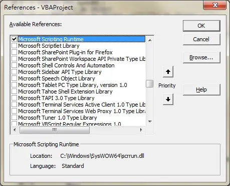
You should be able to run FSO in Excel 2013. If you fail to run FSO Object, open VBE (ALT+F11) > Tools > References > Check the box Microsoft Scripting Runtine

loop_through_workbook

Example – search text in multiple Workbooks in folder

Suppose I want to search text “orange”, “apple”, “pear” in all workbooks under c:\test\, plus workbooks in one level down subfolders under c:\test\

I want to return search result even though the search text is a partial text in a Cell.

For example, if Cell A1 value of a workbook is “Orange Juice”, I still want to return the result because it contains “orange”.

Then create a new workbook that contains the VBA code, change the parameters that highlighted in red. Run the Procedure.

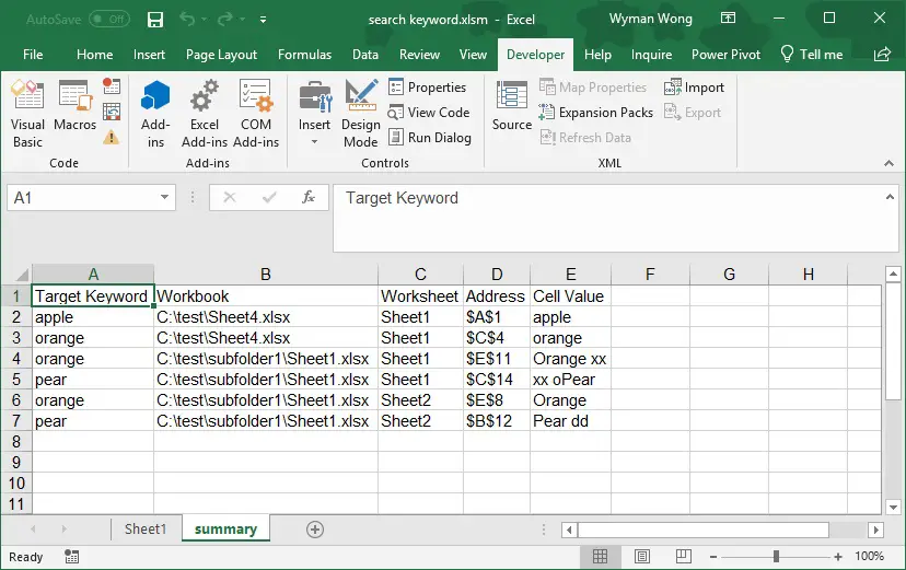
A summary worksheet is created, all the workbooks that contains “apple”, “orange” and “pear” will appear in the summary.
 

MS Access select the first record of each group using First Function

This MS Access tutorial explains how to select the first record of each group using First Function.

MS Access select the first record of each group

When I create human resources report, I have always come across a situation where one employee has more than one records. For example, I want to create a staff list where one employee only has one row of record. If I add emergency contact field to the report and if an employee has more than one emergency contacts, then the Query will return one employees with multi-rows of record as below.

Student IDNameEmergency Contact
1AppleMary
1AppleJohn
2BananaPatrick
2BananaQueenie
3CatAnthony


In order to avoid multiple records of each EE, we have to extract the first record of Emergency Contact for each employee as shown below.

Student IDNameEmergency Contact
1AppleMary
2BananaPatrick
3CatAnthony

Although it is not ideal as the other Emergency Contact is lost in the staff list, it is still the best workaround we can have.

In this post, I will demonstrate how to do it in MS Access.

MS Access select the first record of each group – using First Function

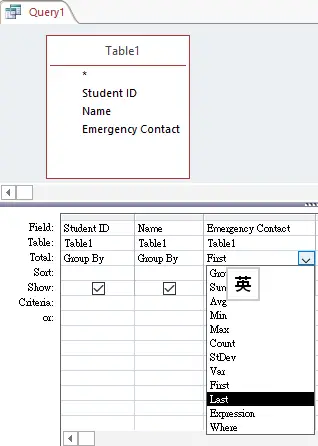
First of all, Group by Student ID and Name (Home > totals icon), then in the Emergency Contact, select aggregate function First, it means after the data is grouped by Student ID, Name, the first record of each group is returned.


Then we get the below result.

Student IDNameEmergency Contact
1AppleMary
2BananaPatrick
3CatAnthony

If you want to apply sorting before selecting the first record, you should create another Query in advance to sort Student ID and Emergency Contact, then the first Emergency Contact changed.


There is also another Function called Last, which select the last record of each group.


Result

Student IDNameEmergency ContactOfLast
1AppleJohn
2BananaQueenie
3CatAnthony

Instead of applying First and Last, you may also consider Min and Max Function. When applying Min and Max, the texts are compared in the same way as sorting text in Excel.

Outbound References

https://support.office.com/en-ie/article/first-last-functions-acd76019-c37f-432d-9807-4fc63cac1db5

How to Change Default Excel Date Format (such as MMDD to DDMM)

This Excel tutorial explains how to change default Excel Date Format from Change Date and Time Format in Control Panel.

How to Change Default Excel Date Format

In the country I live, we normally use date format dd/mm/yyyy. However whenever I work for the US company, the system defaults to mm/dd/yyyy. This is annoying and it causes Excel error. For example, if I mistakenly type UK format 31/12/2019, the date will be recognized as a text because there is no such month as 31. It is even risky if you don’t see this error as you are not aware that you have mistakenly input a wrong date. Although you can simply use Text Function to change the date format, it is just a one time solution and it does not address the issue every time you create a new Workbook.

This tutorial will explain how to change default Excel date format from Windows setting. The change does not just apply to Excel but all the related Windows environment. Note that if you are not a Windows administrator, you may not be able to make this change.

Example – Change Default Excel Date Format in Control Panel

Suppose we want to change default Excel date format from dd/mm/yyyy to mm/dd/yyyy.


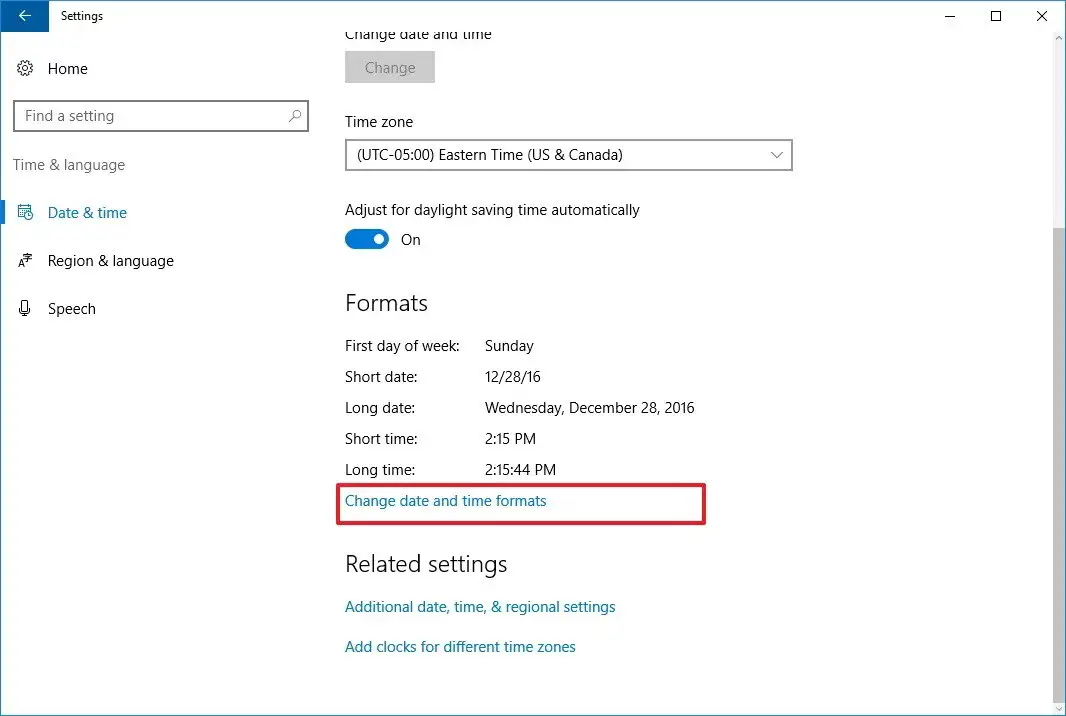
In Windows 10, navigate to Control Panel > Date and Time > Change Date and Time Format

Even if you are using older versions of Windows, the navigation maybe a little bit different, you can still find this option.


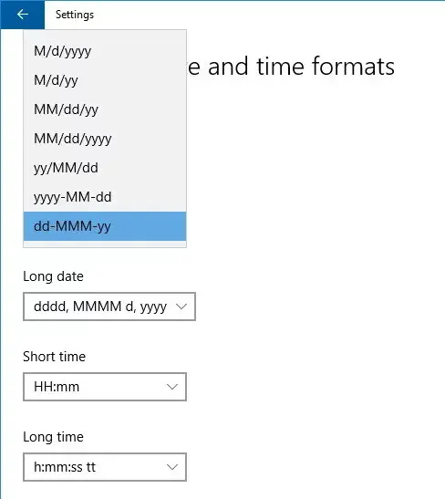
The Short Date format is currently displaying dd/MM/YYYY, now change to MM/dd/yyyy.


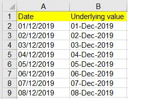
Go back to Excel spreadsheet, the value in column A automatically changed.

This makes complete sense because if the date format doesn’t change, all your existing workbooks will be messed up.

Outbound References

https://support.office.com/en-gb/article/text-function-20d5ac4d-7b94-49fd-bb38-93d29371225c

Group Date and Ungroup Month in Excel Pivot Table

This Excel tutorial explains how to group dates and ungroup month in Excel Pivot Table to prevent auto grouping of Pivot Table in Excel 2016.

Group Date and Ungroup Month in Excel Pivot Table

Since Excel 2016,  when you drag a date field to a Pivot Table Pivot Table Row, the dates are  automatically grouped by months instead of showing each date. This is extremely annoying because  it is tricky to ungroup the months if it is the first time you encounter this issue.

In this post I am going to explain how to ungroup month in Excel Pivot Table and how to group dates by year or month.

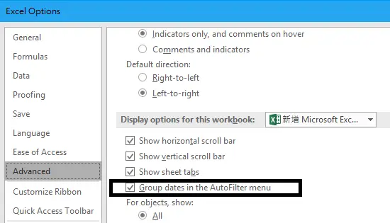
Note that there is an Excel Option called Group dates in the AutoFilter Menu in Excel option, it does not work for Pivot Table Row Grouping. This option is for normal Auto Filter, not Pivot Table, so don’t get confused.

Ungroup Month in Excel Pivot Table

Suppose we have a data source which are dates from 2019 to 2021.


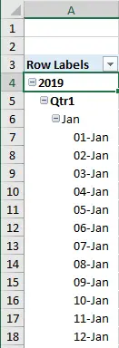
Insert a Pivot Table, and then drag the date field to Rows,the dates are automatically grouped by Year, Quarter and Month by default.

In order to display the original dates without grouping, right click on the data, select Group.

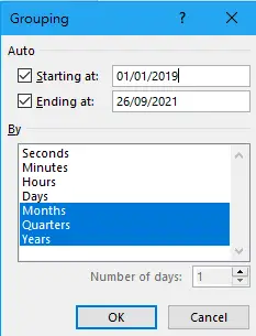
In the dates Grouping options, you can redefine how you want to group the dates. To display the original  dates on each row, highlight Days then OK.

Now the months are ungrouped and are displayed on each row.

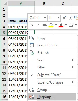
Alternatively, you can simply right click on the date, then select Ungroup. this will ungroup every grouping.

Outbound References

https://support.office.com/en-gb/article/group-or-ungroup-data-in-a-pivottable-c9d1ddd0-6580-47d1-82bc-c84a5a340725

How to convert Excel to PDF

This Excel tutorial explains how to export Excel to PDF in Microsoft Excel and convert Excel to PDF using different online tools.

How to convert Excel to PDF

Excel spreadsheets are widely being used in today’s world in order to manage data. The ability to organize data effectively has contributed a lot towards the popularity of the Excel files. However, the Excel files are not portable and it is not the best method available for you to send out a document. That’s because there is a possibility for the recipient to edit the Excel file. The formatting that you have on the Excel file can also get changed when you are sending it to someone. That’s where you will come across the requirement to convert Excel to PDF.

When you want to convert Excel to PDF, you are provided with a variety of options to consider. It is up to you to go through these options and select the best one out of them. Then you will be able to get an enhanced experience at the end of the day. In fact, you can easily overcome the hassle and pain that is linked with getting the Excel files converted to PDF.

Here is a list of 3 of the best tools, which are available for you to convert Excel to PDF. You can take a look at these tools and settle down with the best option out of them.

Onlineconvertfree.com

Onlineconvertfree.com can be considered as one of the most impressive and innovative tools available for you to convert Excel to PDF. You will be able to get an enhanced experience out of this tool. However, you need to understand that the primary functionality of this tool is not to help you convert Excel to PDF. Instead, it can be considered as a versatile and an all-around converter. You will be able to convert any kind of a file to a supported file format with the assistance that you are getting from onlineconvertfree.com.

The simplicity of onlineconvertfree.com, which you can experience at the time of converting Excel files to PDF files is impressive. You will love the overall conversion process and how it will be able to deliver quick results to you. Onlineconvertfree.com has got a simple and easy to use interface. You can easily upload the raw files that you have into this file converter. Then you will be able to select the output file format. For example, if you upload an Excel file, you can select the output file format as PDF. Then you will be able to get the file converted with minimum hassle. The Excel to PDF conversion process is instant as well and you will be able to end up with outstanding results at the end of the day.

Nova PDF

Nova PDF can be considered as an addon, which you can download to Excel. You can easily integrate this add-on with Excel and then proceed with the file conversion. It is compatible with all the applications that come under Microsoft Office package, including Microsoft Excel and Microsoft PowerPoint. On the other hand, users are provided with the opportunity to create PDF files directly from the Microsoft Excel interface. This can provide a smooth experience.

Once you have configured Nova PDF with Microsoft Excel, which you have installed on your computer, you will be able to see that as a new menu item. You can visit the menu and then click on the option named as “Save As PDF”. Then you will be able to initiate the PDF conversion. The Excel workbook will immediately be converted into a PDF as well and you will be able to experience a smooth conversion. Hence, it is a great option that you can consider.

Export Excel to PDF in Microsoft Excel

Without downloading and configuring any other tool with Microsoft Excel, you are able to get the PDF conversions done as well.

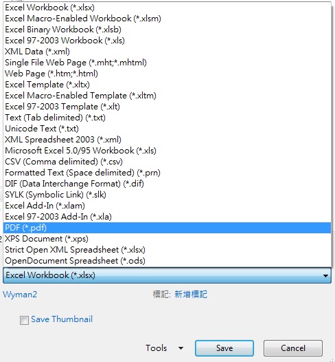
In Excel, navigate to File > Save As, in the Save As Type,  you can save a file as different file types. Below are the available types in Excel 2013.

excel_export_to_pdf


Select PDF, then click on the button Options

excel_export_to_pdf_02


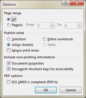
In Options, you can select whether to export Entire workbook to PDF or just Active worksheet(s).

excel_export_to_pdf_03

Note that Entire workbook means all worksheets are exported to one PDF.

Active sheet(s) means to export the selected sheets to one PDF. Normally Active sheet means the worksheet you are currently viewing before you press Save As, but you can hold down Ctrl to select multiple worksheets in order to export specific worksheets to one PDF. Unfortunately there is no built-in option to save each worksheet as separate PDF, but you can refer to my previous post to do it with Excel VBA.

The items in Options are self-explanatory, except there are a few items that require clarification.

Ignore print areasPrint the selection / entire worksheet and ignore print area
Document propertiesInclude title, subject, author, and similar information.
Document structure tags for accessibilityInclude additional data that help disabled users
ISO 19005-1 compliant (PDF/A)A standard of PDF, click here to see details

Outbound Reference

https://support.office.com/en-za/article/Publish-as-PDF-or-XPS-d3b9469c-59ba-49f9-9adf-5707db2451fa?ui=en-US&rs=en-ZA&ad=ZA


Access VBA delete Table records with SQL using DoCMD.RunSQL Method

This Access VBA tutorial explains how to use VBA delete Table records with SQL without alert using DoCMD.RunSQL Method.

You may also want to read:

Access VBA run Query or run Action Query

Access delete Table records

In my previous post, I have explained how to delete Table records without using VBA, below is a quick recap.

Suppose we have created a table called student in Access, which contains 5 student records.

student
Student IDStudent Name
001Apple
002Betty
003Cathy
004David
005Elyse

In order to delete the record (the whole row) of Apple, create a new Query, add student table.

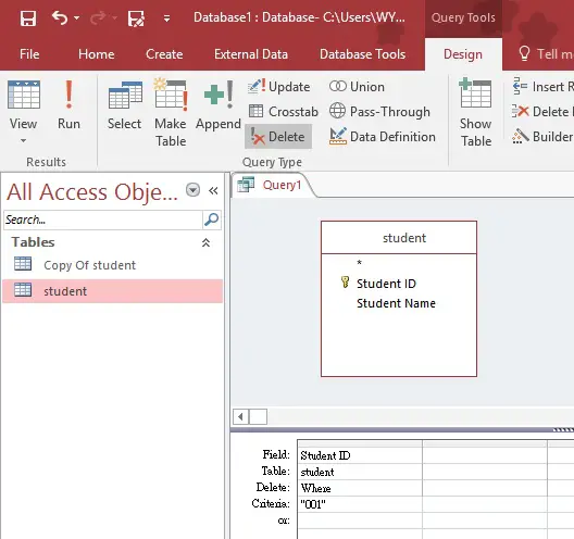
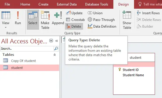
Under Design tab, click on Delete button. This will create a Delete Query.
access-delete-table-records-01


Add Student ID to the field, then type “001” in criteria, which is the student ID of Apple.

access-delete-table-records-02


To preview the result of Delete Query (which records will be deleted), click on the View button under Design.

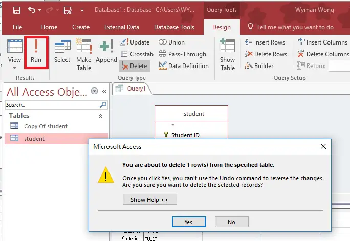
To execute the Query (actually delete the records), click on Run button, then click on Yes to confirm delete row.

access-delete-table-records-03


Access VBA delete Table records

Similar to executing Delete Query in Access UI, you can delete Access Table records in VBA. First write a standard Delete SQL statement, then use DoCMD.RunSQL Method to execute the SQL.

For example, we have a student Table as below.

student
Student IDStudent Name
001Apple
002Betty
003Cathy
004David
005Elyse


Press ALT+F11 and insert the below code in Module.

Public Sub deleteRecord()
    DoCmd.SetWarnings False
    strSQL = "Delete * From [student] WHERE [Student ID]='002'"
    DoCmd.RunSQL strSQL
    DoCmd.SetWarnings True
End Sub

Writing DoCmd.SetWarings False is because we want to avoid Access generating the below Alert so that the subsequent statements can be executed smoothly.


Run the Sub, then you will see the below result where Student ID 002 is deleted.
student
Student IDStudent Name
001Apple
003Cathy
004David
005Elyse


Outbound References

https://docs.microsoft.com/en-us/office/vba/api/access.docmd.runsql

VBA Excel Access roundup rounddown Function

This Excel Access tutorial explains how to use VBA to write an Access roundup (round up) and Access rounddown (round down) Function to simulate that in Excel. These roundup and rounddown Functions can also be used in Access and Excel VBA.

Excel Access roundup rounddown Function

In Excel Worksheet Function, there are round, roundup, rounddown, mround Functions.

In Excel VBA, there is only round Function but no roundup, rounddown, mround Functions. The round Function is not the same as that in Excel Worksheet Function, the round logic that is being used is called Round-To-Even logic. However, you can still access Worksheet Functions in Excel VBA with WorksheetFunction Method as below.

In Microsoft Access (VBA / application) there is only round function that uses Round-To-Even logic. Therefore, there is a need to recreate round, roundup, rounddown, mround Functions in VBA, no matter in Access or Excel VBA. In my previous posts, I have written VBA Function to simulate Excel mround and round Functions. In this post, I will write roundup and rounddown Functions.

VBA Code – Excel Access roundup Function

Public Function wRoundUp(pValue, digit) As Double
    ExpandedValue = Abs(pValue) * (10 ^ digit) 'Retrieve integer part of the number
    wRoundUp = Sgn(pValue) * Int(ExpandedValue + 0.99999999) / 10 ^ digit
End Function

Explanation

This Excel Access roundup Function performs two major actions. First, the target number is expanded to the decimal places which you want to round up, and then add 0.9999999 to the number, so that it goes up to the next integer. Finally use INT Function to extract the integer part. The sign of the number is ignored during round up and down to simulate the behavior in Excel, then it is added back after rounding.

For example, we have a number 14.56 and we want to round up to 1 decimal places. 14.56 is first expanded to 145.6, and then add 0.9999999, so that it becomes something like 146.6. Finally extract the integer part (146), divided by 100 to become 14.6.

VBA Code – Excel Access rounddown Function

Public Function wRoundDown(pValue, digit) As Double
    ExpandedValue = Abs(pValue) * (10 ^ digit) 'Retrieve integer part of the number
    wRoundDown = Sgn(pValue) * Int(ExpandedValue) / 10 ^ digit
End Function

Explanation

This Excel Access rounddown Function performs two major actions. First, the target number is expanded to the decimal places which you want to round up, then we use INT Function to extract the integer part. The sign of the number is ignored during round up and down to simulate the behavior in Excel, then it is added back after rounding.

For example, we have a number 14.56 and we want to round down to 1 decimal places. 14.56 is first expanded to 145.6, and then we extract only 145. Finally divided by 10 to become 14.5.

Example – roundup and rounddown

FormulaResult
wROUNDUP(1.113,2)1.12
wROUNDDOWN(1.112,1)1.1
wROUNDUP(1.094,2)1.1
wROUNDDOWN(1.093,1)1
wROUNDUP(-1.113,2)-1.12
wROUNDDOWN(-1.112,1)-1.1
wROUNDUP(-1.094,2)-1.1
wROUNDDOWN(-1.093,1)-1