This Excel tutorial explains how to use Share Workbook function to allow multiple users to open the workbook at the same time.
Excel Share Workbook
Share Workbook function allows multiple users to open the workbook at the same time.
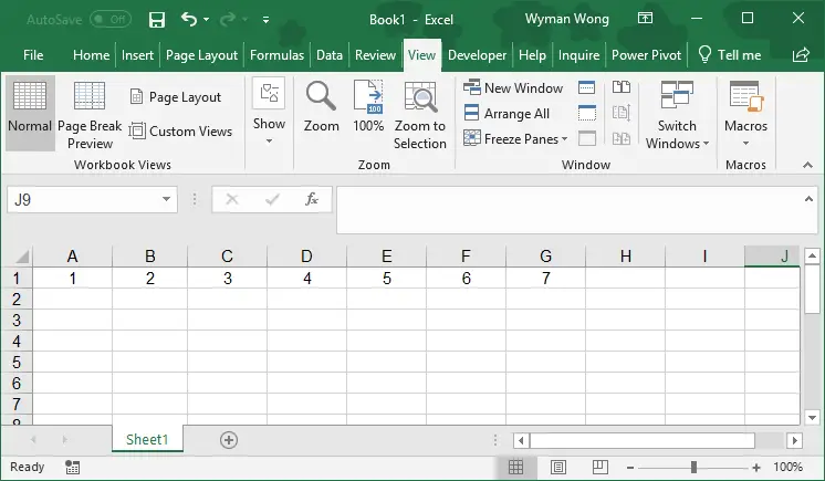
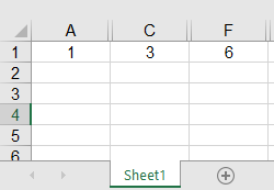
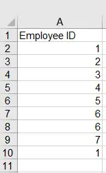
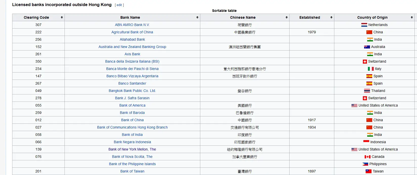
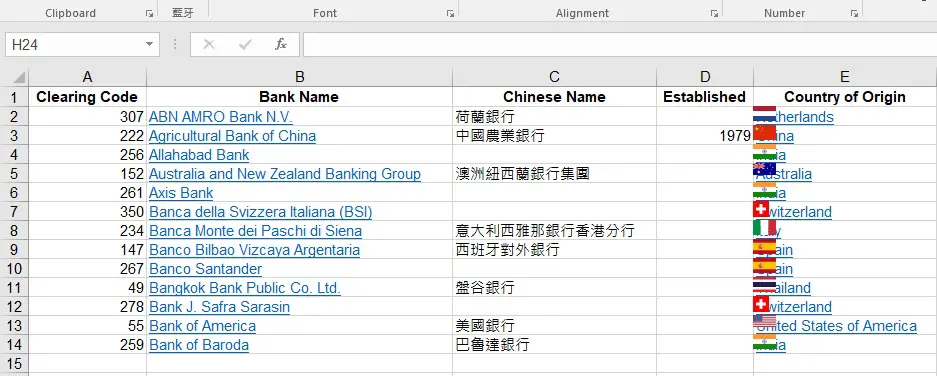
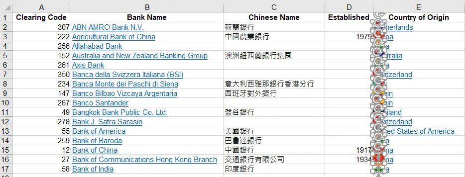
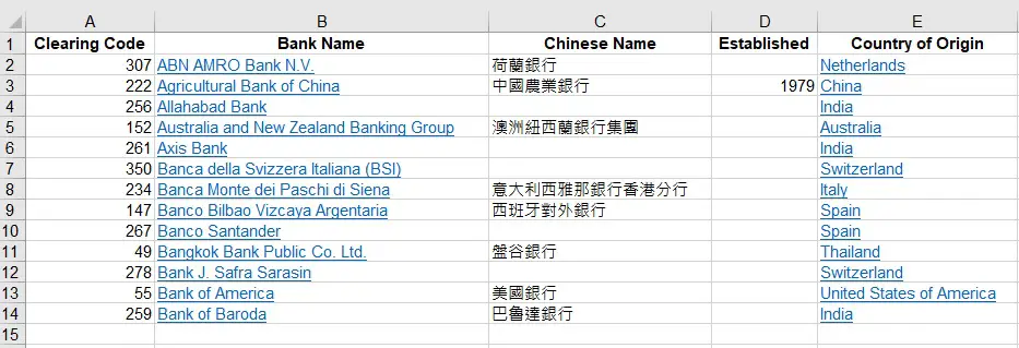
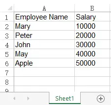
Assume that we have a staff list workbook that is placed in the network share drive.

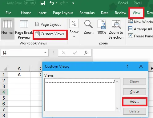
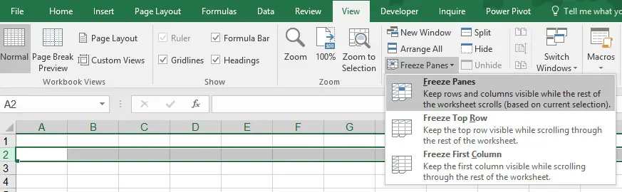
Click on REVIEW > Share Workbook

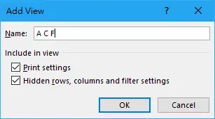
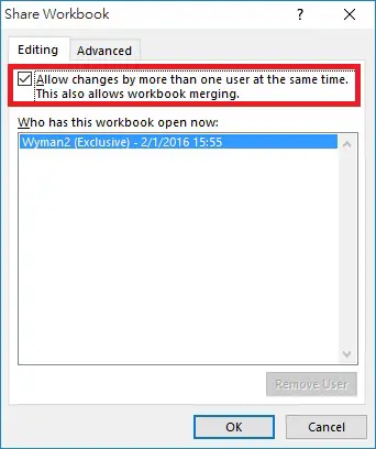
Check the box “Allow changes by more than one user at the same time. This also allows workbook merging” > OK

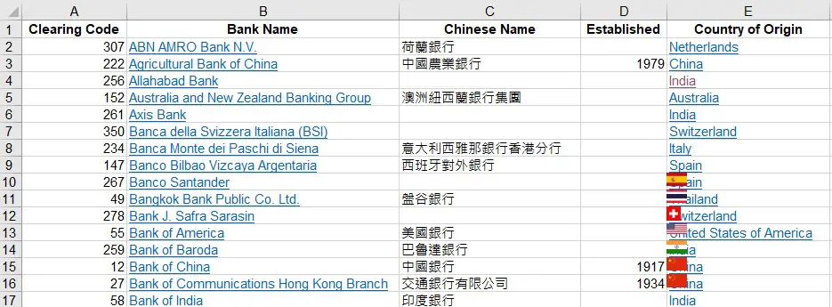
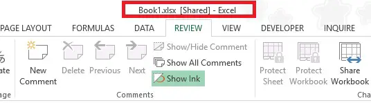
Now you can see the workbook name has [Shared] in the suffix

Modify Share Workbook by others
Lets say the computer we just used to share workbook is called Workstation1, now we are going to open the workbook from another network computer called Workstation2.
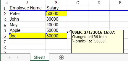
Delete row 2 (Mary), modify Peter’s salary, add one more row of data for Joe in the last row. Save the workbook.

Go back to workstation1, save the workbook, now you can see the workbook is updated with values changed by workstation2. Changes are also highlighted in blue color with comments inserted.

Review changes of Share Workbook made by others
Hover the mouse over the comments to see the old value and new value change.

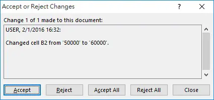
Click on REVIEW > Track Changes > Accept/Reject Changes

Click on Accept to accept the change the those highlighted changes will be gone.
Click on Reject to change back to the original value.
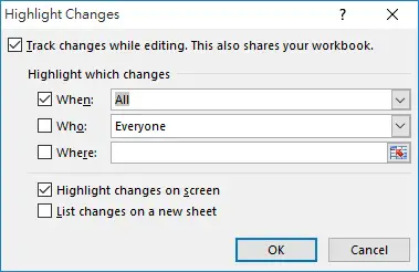
If you cannot see the highlighted changes or you want to see the historical changes, click on REVIEW > Track Changes > Highlight Changes

Now you can see the previous changes again
Other options of Share Workbook
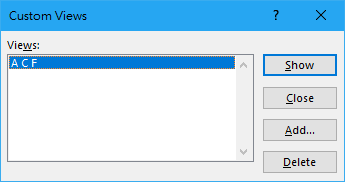
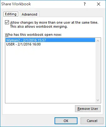
Click on REVIEW > Shareworkbook
You can see who are currently opening the workbook. — USER is workstation2 in our case.
You can click on Remove User to kick the user out of the share workbook. Once the user being kicked save the workbook, a notification will pop up telling them no changes will be made to the the share workbook and suggest them to save the workbook as another file.
Click on the Advanced tab to see how you would like to keep the change history, and also how to deal with conflicting changes when users edit on the same cells.
Conflicting Changes for option “Ask me which changes win”
Lets say Workstation1 changes B4 value to 100000, then save the workbook. Then Workstation2 changes the value to 200000, save the workbook, a Windows will pop up in Workstation2 asking if you want to kept your change or accept other’s change.

Stop Share Workbook
Click on REVIEW > Shareworkbook > uncheck the box > OK
Disconnected from Share Workbook
No matter whether you are disconnected due to network issue or being kicked out, in that case you need to know what changes you have made but not updated in the Share Workbook.
Read my another post to compare workbook in order to find out the updates you need to move to the Share Workbook.
Excel VBA compare worksheets
Excel Compare Worksheets using Compare File
Features not supported in Share Workbook
I refer to the Microsoft documentation in the below section.
Not all features are supported in a shared workbook. If you want to include any of the following features, you should add them before you save the workbook as a shared workbook: merged cells, conditional formats, data validation, charts, pictures, objects including drawing objects, hyperlinks, scenarios, outlines, subtotals, data tables, PivotTable reports, workbook and worksheet protection, and macros. You cannot make changes to these features after you share the workbook.
Features that are not supported in a shared workbook
| In a shared workbook, you cannot | But you may be able to do the following |
| Create an Excel table | None |
| Insert or delete blocks of cells | You can insert entire rows and columns. |
| Delete worksheets | None |
| Merge cells or split merged cells | None |
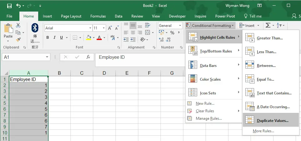
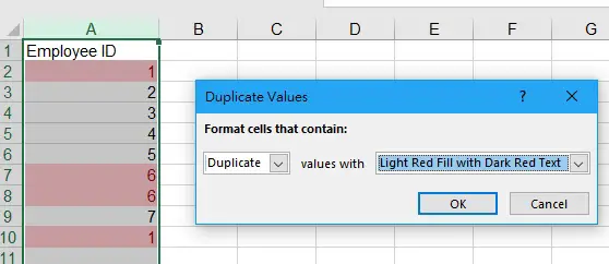
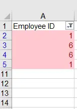
| Add or change conditional formats | Existing conditional formats continue to appear as cell values change, but you can’t change these formats or redefine the conditions. |
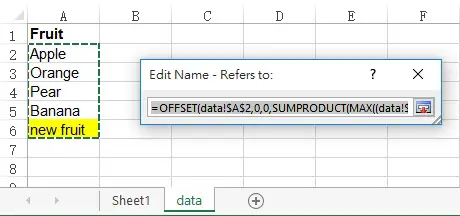
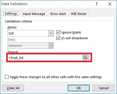
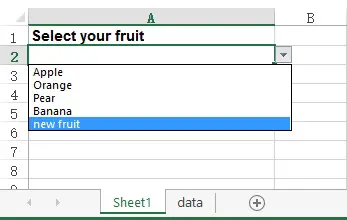
| Add or change data validation | Cells continue to be validated when you type new values, but you can’t change existing data validation settings. |
| Create or change charts or PivotChart reports | You can view existing charts and reports. |
| Insert or change pictures or other objects | You can view existing pictures and objects. |
| Insert or change hyperlinks | Existing hyperlinks continue to work. |
| Use drawing tools | You can view existing drawings and graphics. |
| Assign, change, or remove passwords | Existing passwords remain in effect. |
| Protect or unprotect worksheets or the workbook | Existing protection remains in effect. |
| Create, change, or view scenarios | None |
| Group or outline data | You can continue to use existing outlines. |
| Insert automatic subtotals | You can view existing subtotals. |
| Create data tables | You can view existing data tables. |
| Create or change PivotTable reports | You can view existing reports. |
| Write, record, change, view, or assign macros | You can run existing macros that don’t access unavailable features. You can record shared workbook operations into a macro stored in another nonshared workbook. |
| Add or change Microsoft Excel 4 dialog sheets | None |
| Change or delete array formulas | Existing array formulas continue to calculate correctly. |
| Use a data form to add new data | You can use a data form to find a record. |
Work with XML data, including:- Import, refresh, and export XML data
- Add, rename, or delete XML maps
- Map cells to XML elements
- Use the XML Source task pane, XML toolbar, or XML commands on the Data menu
| None |